Free Statistics
of Irreproducible Research!
Description of Statistical Computation | |||||||||||||||||||||||||||||||||||||
|---|---|---|---|---|---|---|---|---|---|---|---|---|---|---|---|---|---|---|---|---|---|---|---|---|---|---|---|---|---|---|---|---|---|---|---|---|---|
| Author's title | |||||||||||||||||||||||||||||||||||||
| Author | *The author of this computation has been verified* | ||||||||||||||||||||||||||||||||||||
| R Software Module | rwasp_boxcoxnorm.wasp | ||||||||||||||||||||||||||||||||||||
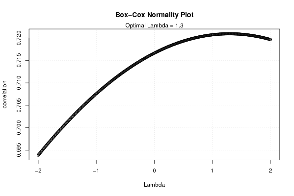
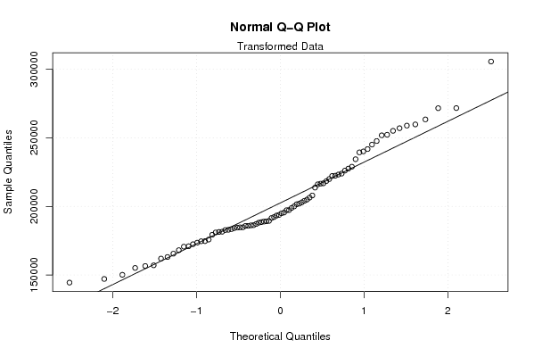
| Title produced by software | Box-Cox Normality Plot | ||||||||||||||||||||||||||||||||||||
| Date of computation | Sun, 14 Dec 2008 07:53:59 -0700 | ||||||||||||||||||||||||||||||||||||
| Cite this page as follows | Statistical Computations at FreeStatistics.org, Office for Research Development and Education, URL https://freestatistics.org/blog/index.php?v=date/2008/Dec/14/t1229266533ib2obkoae1wu1pl.htm/, Retrieved Thu, 16 May 2024 02:16:17 +0000 | ||||||||||||||||||||||||||||||||||||
| Statistical Computations at FreeStatistics.org, Office for Research Development and Education, URL https://freestatistics.org/blog/index.php?pk=33404, Retrieved Thu, 16 May 2024 02:16:17 +0000 | |||||||||||||||||||||||||||||||||||||
| QR Codes: | |||||||||||||||||||||||||||||||||||||
|
| |||||||||||||||||||||||||||||||||||||
| Original text written by user: | |||||||||||||||||||||||||||||||||||||
| IsPrivate? | No (this computation is public) | ||||||||||||||||||||||||||||||||||||
| User-defined keywords | |||||||||||||||||||||||||||||||||||||
| Estimated Impact | 145 | ||||||||||||||||||||||||||||||||||||
Tree of Dependent Computations | |||||||||||||||||||||||||||||||||||||
| Family? (F = Feedback message, R = changed R code, M = changed R Module, P = changed Parameters, D = changed Data) | |||||||||||||||||||||||||||||||||||||
| - [Box-Cox Normality Plot] [Invoer] [2008-12-14 14:53:59] [5925747fb2a6bb4cfcd8015825ee5e92] [Current] | |||||||||||||||||||||||||||||||||||||
| Feedback Forum | |||||||||||||||||||||||||||||||||||||
Post a new message | |||||||||||||||||||||||||||||||||||||
Dataset | |||||||||||||||||||||||||||||||||||||
| Dataseries X: | |||||||||||||||||||||||||||||||||||||
11554,5 13182,1 14800,1 12150,7 14478,2 13253,9 12036,8 12653,2 14035,4 14571,4 15400,9 14283,2 14485,3 14196,3 15559,1 13767,4 14634 14381,1 12509,9 12122,3 13122,3 13908,7 13456,5 12441,6 12953 13057,2 14350,1 13830,2 13755,5 13574,4 12802,6 11737,3 13850,2 15081,8 13653,3 14019,1 13962 13768,7 14747,1 13858,1 13188 13693,1 12970 11392,8 13985,2 14994,7 13584,7 14257,8 13553,4 14007,3 16535,8 14721,4 13664,6 16805,9 13829,4 13735,6 15870,5 15962,4 15744,1 16083,7 14863,9 15533,1 17473,1 15925,5 15573,7 17495 14155,8 14913,9 17250,4 15879,8 17647,8 17749,9 17111,8 16934,8 20280 16238,2 17896,1 18089,3 15660 16162,4 17850,1 18520,4 18524,7 16843,7 | |||||||||||||||||||||||||||||||||||||
Tables (Output of Computation) | |||||||||||||||||||||||||||||||||||||
| |||||||||||||||||||||||||||||||||||||
Figures (Output of Computation) | |||||||||||||||||||||||||||||||||||||
Input Parameters & R Code | |||||||||||||||||||||||||||||||||||||
| Parameters (Session): | |||||||||||||||||||||||||||||||||||||
| Parameters (R input): | |||||||||||||||||||||||||||||||||||||
| R code (references can be found in the software module): | |||||||||||||||||||||||||||||||||||||
n <- length(x) | |||||||||||||||||||||||||||||||||||||