Repository of Reproducible Computations

Free Statistics

of Irreproducible Research!

Author's title

Author

*The author of this computation has been verified*

R Software Module

rwasp_autocorrelation.wasp

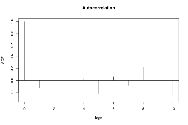
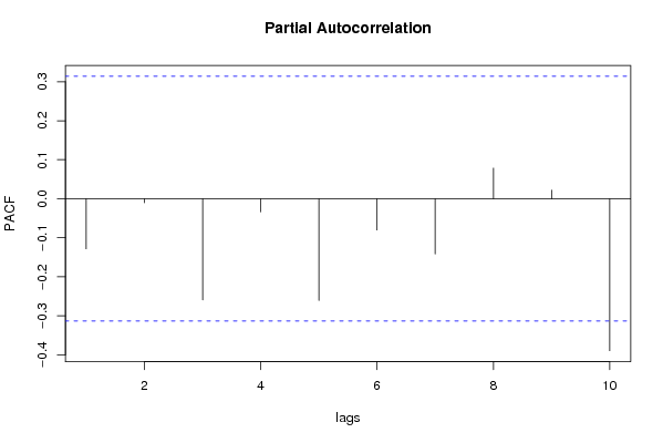
Title produced by software

(Partial) Autocorrelation Function

Date of computation

Sun, 14 Dec 2008 07:21:15 -0700

Cite this page as follows

Statistical Computations at FreeStatistics.org, Office for Research Development and Education, URL https://freestatistics.org/blog/index.php?v=date/2008/Dec/14/t1229264535hy2ok4tvxhobdww.htm/, Retrieved Wed, 15 May 2024 16:18:46 +0000

Statistical Computations at FreeStatistics.org, Office for Research Development and Education, URL https://freestatistics.org/blog/index.php?pk=33391, Retrieved Wed, 15 May 2024 16:18:46 +0000

QR Codes:

Paste this QR Code to cite your computation.

Original text written by user:

IsPrivate?

No (this computation is public)

User-defined keywords

Estimated Impact

181

Family? (F = Feedback message, R = changed R code, M = changed R Module, P = changed Parameters, D = changed Data)

-     [(Partial) Autocorrelation Function] [VAC (Parti�le) au...] [2008-12-14 13:47:12] [379d6c32f73e3218fd773d79e4063d07]
-    D    [(Partial) Autocorrelation Function] [VAC (Parti�le) au...] [2008-12-14 14:21:15] [490fee4f334e2e025c95681783e3fd0b] [Current]
- RM D      [Cross Correlation Function] [VAC cross correla...] [2008-12-14 14:31:56] [379d6c32f73e3218fd773d79e4063d07] 
-   PD        [Cross Correlation Function] [VAC cross correla...] [2008-12-23 15:12:44] [379d6c32f73e3218fd773d79e4063d07] 
-  M            [Cross Correlation Function] [Cross Cerelation ...] [2010-01-23 19:21:52] [f1bd7399181c649098ca7b814ee0e027] 
- RM        [ARIMA Backward Selection] [VAC Arima backwar...] [2008-12-14 14:58:49] [379d6c32f73e3218fd773d79e4063d07] 
- RM D      [ARIMA Backward Selection] [VAC Arima backwar...] [2008-12-14 15:01:07] [379d6c32f73e3218fd773d79e4063d07] 
-   PD        [ARIMA Backward Selection] [VAC Arima backwar...] [2008-12-17 11:54:33] [379d6c32f73e3218fd773d79e4063d07] 
-   PD          [ARIMA Backward Selection] [VAC Arima backwar...] [2008-12-17 13:12:49] [379d6c32f73e3218fd773d79e4063d07] 
-   PD            [ARIMA Backward Selection] [VAC Arima backwar...] [2008-12-23 15:36:28] [379d6c32f73e3218fd773d79e4063d07] 
-  MP               [ARIMA Backward Selection] [ARIMA Backward Se...] [2010-01-23 19:27:59] [f1bd7399181c649098ca7b814ee0e027] 
-               [ARIMA Backward Selection] [VAC Arima backwar...] [2008-12-23 15:24:00] [379d6c32f73e3218fd773d79e4063d07] 
-  MP             [ARIMA Backward Selection] [ARIMA Backward Se...] [2010-01-23 19:26:35] [f1bd7399181c649098ca7b814ee0e027] 
-               [ARIMA Backward Selection] [VAC Arima backwar...] [2008-12-23 16:01:32] [379d6c32f73e3218fd773d79e4063d07] 

Feedback Forum

Post a new message

Dataseries X:

Download CSV

Histogram

Boxplots

Summary of computational transaction
Raw Input	view raw input (R code)
Raw Output	view raw output of R engine
Computing time	1 seconds
R Server	'George Udny Yule' @ 72.249.76.132

\begin{tabular}{lllllllll}
\hline
Summary of computational transaction \tabularnewline
Raw Input & view raw input (R code)  \tabularnewline
Raw Output & view raw output of R engine  \tabularnewline
Computing time & 1 seconds \tabularnewline
R Server & 'George Udny Yule' @ 72.249.76.132 \tabularnewline
\hline
\end{tabular}
%Source: https://freestatistics.org/blog/index.php?pk=33391&T=0

[TABLE]
[ROW][C]Summary of computational transaction[/C][/ROW]
[ROW][C]Raw Input[/C][C]view raw input (R code) [/C][/ROW]
[ROW][C]Raw Output[/C][C]view raw output of R engine [/C][/ROW]
[ROW][C]Computing time[/C][C]1 seconds[/C][/ROW]
[ROW][C]R Server[/C][C]'George Udny Yule' @ 72.249.76.132[/C][/ROW]
[/TABLE]
Source: https://freestatistics.org/blog/index.php?pk=33391&T=0

Globally Unique Identifier (entire table): ba.freestatistics.org/blog/index.php?pk=33391&T=0

As an alternative you can also use a QR Code:

The GUIDs for individual cells are displayed in the table below:

Summary of computational transaction
Raw Input	view raw input (R code)
Raw Output	view raw output of R engine
Computing time	1 seconds
R Server	'George Udny Yule' @ 72.249.76.132

Autocorrelation Function
Time lag k	ACF(k)	T-STAT	P-value
1	-0.128413	-0.8019	0.213724
2	0.00637	0.0398	0.484237
3	-0.25456	-1.5897	0.059986
4	0.03575	0.2233	0.41225
5	-0.229986	-1.4363	0.079451
6	0.065068	0.4063	0.343354
7	-0.085367	-0.5331	0.298488
8	0.228507	1.427	0.080765
9	0.002105	0.0131	0.494789
10	-0.251785	-1.5724	0.061969

\begin{tabular}{lllllllll}
\hline
Autocorrelation Function \tabularnewline
Time lag k & ACF(k) & T-STAT & P-value \tabularnewline
1 & -0.128413 & -0.8019 & 0.213724 \tabularnewline
2 & 0.00637 & 0.0398 & 0.484237 \tabularnewline
3 & -0.25456 & -1.5897 & 0.059986 \tabularnewline
4 & 0.03575 & 0.2233 & 0.41225 \tabularnewline
5 & -0.229986 & -1.4363 & 0.079451 \tabularnewline
6 & 0.065068 & 0.4063 & 0.343354 \tabularnewline
7 & -0.085367 & -0.5331 & 0.298488 \tabularnewline
8 & 0.228507 & 1.427 & 0.080765 \tabularnewline
9 & 0.002105 & 0.0131 & 0.494789 \tabularnewline
10 & -0.251785 & -1.5724 & 0.061969 \tabularnewline
\hline
\end{tabular}
%Source: https://freestatistics.org/blog/index.php?pk=33391&T=1

[TABLE]
[ROW][C]Autocorrelation Function[/C][/ROW]
[ROW][C]Time lag k[/C][C]ACF(k)[/C][C]T-STAT[/C][C]P-value[/C][/ROW]
[ROW][C]1[/C][C]-0.128413[/C][C]-0.8019[/C][C]0.213724[/C][/ROW]
[ROW][C]2[/C][C]0.00637[/C][C]0.0398[/C][C]0.484237[/C][/ROW]
[ROW][C]3[/C][C]-0.25456[/C][C]-1.5897[/C][C]0.059986[/C][/ROW]
[ROW][C]4[/C][C]0.03575[/C][C]0.2233[/C][C]0.41225[/C][/ROW]
[ROW][C]5[/C][C]-0.229986[/C][C]-1.4363[/C][C]0.079451[/C][/ROW]
[ROW][C]6[/C][C]0.065068[/C][C]0.4063[/C][C]0.343354[/C][/ROW]
[ROW][C]7[/C][C]-0.085367[/C][C]-0.5331[/C][C]0.298488[/C][/ROW]
[ROW][C]8[/C][C]0.228507[/C][C]1.427[/C][C]0.080765[/C][/ROW]
[ROW][C]9[/C][C]0.002105[/C][C]0.0131[/C][C]0.494789[/C][/ROW]
[ROW][C]10[/C][C]-0.251785[/C][C]-1.5724[/C][C]0.061969[/C][/ROW]
[/TABLE]
Source: https://freestatistics.org/blog/index.php?pk=33391&T=1

Globally Unique Identifier (entire table): ba.freestatistics.org/blog/index.php?pk=33391&T=1

As an alternative you can also use a QR Code:

The GUIDs for individual cells are displayed in the table below:

Autocorrelation Function
Time lag k	ACF(k)	T-STAT	P-value
1	-0.128413	-0.8019	0.213724
2	0.00637	0.0398	0.484237
3	-0.25456	-1.5897	0.059986
4	0.03575	0.2233	0.41225
5	-0.229986	-1.4363	0.079451
6	0.065068	0.4063	0.343354
7	-0.085367	-0.5331	0.298488
8	0.228507	1.427	0.080765
9	0.002105	0.0131	0.494789
10	-0.251785	-1.5724	0.061969

Partial Autocorrelation Function
Time lag k	PACF(k)	T-STAT	P-value
1	-0.128413	-0.8019	0.213724
2	-0.01029	-0.0643	0.474545
3	-0.259359	-1.6197	0.056679
4	-0.033774	-0.2109	0.417023
5	-0.26103	-1.6301	0.055562
6	-0.080334	-0.5017	0.309354
7	-0.141556	-0.884	0.191053
8	0.078409	0.4897	0.313558
9	0.021923	0.1369	0.445904
10	-0.389688	-2.4336	0.009816

\begin{tabular}{lllllllll}
\hline
Partial Autocorrelation Function \tabularnewline
Time lag k & PACF(k) & T-STAT & P-value \tabularnewline
1 & -0.128413 & -0.8019 & 0.213724 \tabularnewline
2 & -0.01029 & -0.0643 & 0.474545 \tabularnewline
3 & -0.259359 & -1.6197 & 0.056679 \tabularnewline
4 & -0.033774 & -0.2109 & 0.417023 \tabularnewline
5 & -0.26103 & -1.6301 & 0.055562 \tabularnewline
6 & -0.080334 & -0.5017 & 0.309354 \tabularnewline
7 & -0.141556 & -0.884 & 0.191053 \tabularnewline
8 & 0.078409 & 0.4897 & 0.313558 \tabularnewline
9 & 0.021923 & 0.1369 & 0.445904 \tabularnewline
10 & -0.389688 & -2.4336 & 0.009816 \tabularnewline
\hline
\end{tabular}
%Source: https://freestatistics.org/blog/index.php?pk=33391&T=2

[TABLE]
[ROW][C]Partial Autocorrelation Function[/C][/ROW]
[ROW][C]Time lag k[/C][C]PACF(k)[/C][C]T-STAT[/C][C]P-value[/C][/ROW]
[ROW][C]1[/C][C]-0.128413[/C][C]-0.8019[/C][C]0.213724[/C][/ROW]
[ROW][C]2[/C][C]-0.01029[/C][C]-0.0643[/C][C]0.474545[/C][/ROW]
[ROW][C]3[/C][C]-0.259359[/C][C]-1.6197[/C][C]0.056679[/C][/ROW]
[ROW][C]4[/C][C]-0.033774[/C][C]-0.2109[/C][C]0.417023[/C][/ROW]
[ROW][C]5[/C][C]-0.26103[/C][C]-1.6301[/C][C]0.055562[/C][/ROW]
[ROW][C]6[/C][C]-0.080334[/C][C]-0.5017[/C][C]0.309354[/C][/ROW]
[ROW][C]7[/C][C]-0.141556[/C][C]-0.884[/C][C]0.191053[/C][/ROW]
[ROW][C]8[/C][C]0.078409[/C][C]0.4897[/C][C]0.313558[/C][/ROW]
[ROW][C]9[/C][C]0.021923[/C][C]0.1369[/C][C]0.445904[/C][/ROW]
[ROW][C]10[/C][C]-0.389688[/C][C]-2.4336[/C][C]0.009816[/C][/ROW]
[/TABLE]
Source: https://freestatistics.org/blog/index.php?pk=33391&T=2

Globally Unique Identifier (entire table): ba.freestatistics.org/blog/index.php?pk=33391&T=2

As an alternative you can also use a QR Code:

The GUIDs for individual cells are displayed in the table below:

Partial Autocorrelation Function
Time lag k	PACF(k)	T-STAT	P-value
1	-0.128413	-0.8019	0.213724
2	-0.01029	-0.0643	0.474545
3	-0.259359	-1.6197	0.056679
4	-0.033774	-0.2109	0.417023
5	-0.26103	-1.6301	0.055562
6	-0.080334	-0.5017	0.309354
7	-0.141556	-0.884	0.191053
8	0.078409	0.4897	0.313558
9	0.021923	0.1369	0.445904
10	-0.389688	-2.4336	0.009816

Figure 1

PNG link

Postscript link

PDF link

Figure 2

PNG link

Postscript link

PDF link

Parameters (Session):

par1 = Default ; par2 = 1.1 ; par3 = 1 ; par4 = 1 ; par5 = 4 ;

Parameters (R input):

par1 = 10 ; par2 = 0.3 ; par3 = 1 ; par4 = 0 ; par5 = 4 ;

R code (references can be found in the software module):

if (par1 == 'Default') {
par1 = 10*log10(length(x))
} else {
par1 <- as.numeric(par1)
}
par2 <- as.numeric(par2)
par3 <- as.numeric(par3)
par4 <- as.numeric(par4)
par5 <- as.numeric(par5)
if (par2 == 0) {
x <- log(x)
} else {
x <- (x ^ par2 - 1) / par2
}
if (par3 > 0) x <- diff(x,lag=1,difference=par3)
if (par4 > 0) x <- diff(x,lag=par5,difference=par4)
bitmap(file='pic1.png')
racf <- acf(x,par1,main='Autocorrelation',xlab='lags',ylab='ACF')
dev.off()
bitmap(file='pic2.png')
rpacf <- pacf(x,par1,main='Partial Autocorrelation',xlab='lags',ylab='PACF')
dev.off()
(myacf <- c(racf$acf))
(mypacf <- c(rpacf$acf))
lengthx <- length(x)
sqrtn <- sqrt(lengthx)
load(file='createtable')
a<-table.start()
a<-table.row.start(a)
a<-table.element(a,'Autocorrelation Function',4,TRUE)
a<-table.row.end(a)
a<-table.row.start(a)
a<-table.element(a,'Time lag k',header=TRUE)
a<-table.element(a,hyperlink('basics.htm','ACF(k)','click here for more information about the Autocorrelation Function'),header=TRUE)
a<-table.element(a,'T-STAT',header=TRUE)
a<-table.element(a,'P-value',header=TRUE)
a<-table.row.end(a)
for (i in 2:(par1+1)) {
a<-table.row.start(a)
a<-table.element(a,i-1,header=TRUE)
a<-table.element(a,round(myacf[i],6))
mytstat <- myacf[i]*sqrtn
a<-table.element(a,round(mytstat,4))
a<-table.element(a,round(1-pt(abs(mytstat),lengthx),6))
a<-table.row.end(a)
}
a<-table.end(a)
table.save(a,file='mytable.tab')
a<-table.start()
a<-table.row.start(a)
a<-table.element(a,'Partial Autocorrelation Function',4,TRUE)
a<-table.row.end(a)
a<-table.row.start(a)
a<-table.element(a,'Time lag k',header=TRUE)
a<-table.element(a,hyperlink('basics.htm','PACF(k)','click here for more information about the Partial Autocorrelation Function'),header=TRUE)
a<-table.element(a,'T-STAT',header=TRUE)
a<-table.element(a,'P-value',header=TRUE)
a<-table.row.end(a)
for (i in 1:par1) {
a<-table.row.start(a)
a<-table.element(a,i,header=TRUE)
a<-table.element(a,round(mypacf[i],6))
mytstat <- mypacf[i]*sqrtn
a<-table.element(a,round(mytstat,4))
a<-table.element(a,round(1-pt(abs(mytstat),lengthx),6))
a<-table.row.end(a)
}
a<-table.end(a)
table.save(a,file='mytable1.tab')

Free Statistics

Description of Statistical Computation

Tree of Dependent Computations

Dataset

Tables (Output of Computation)

Figures (Output of Computation)

Input Parameters & R Code