Free Statistics
of Irreproducible Research!
Description of Statistical Computation | |||||||||||||||||||||
|---|---|---|---|---|---|---|---|---|---|---|---|---|---|---|---|---|---|---|---|---|---|
| Author's title | Paper: Trivariate scatterplot Uitvoer Amerika-Prijzen uitvoer-Wisselkoers d... | ||||||||||||||||||||
| Author | *The author of this computation has been verified* | ||||||||||||||||||||
| R Software Module | rwasp_cloud.wasp | ||||||||||||||||||||
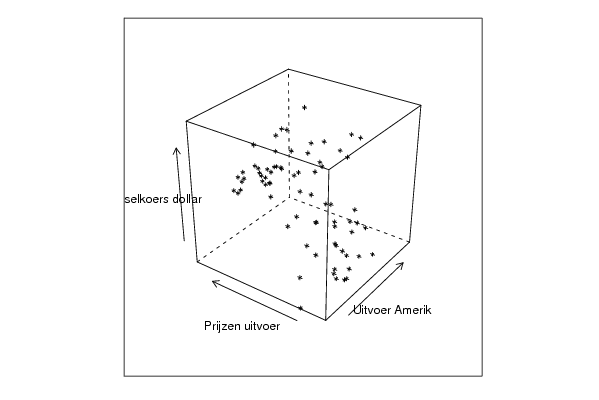
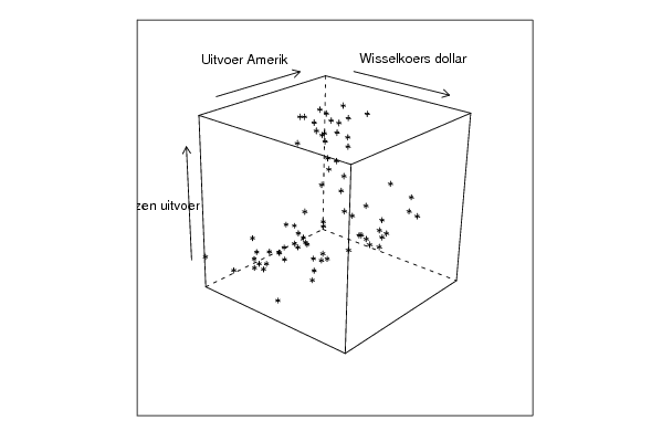
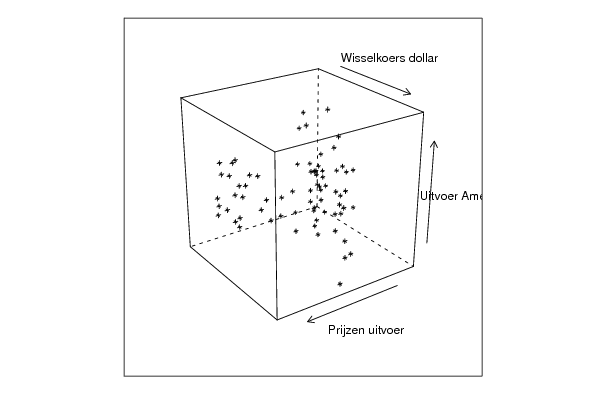
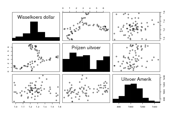
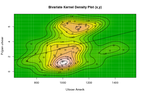
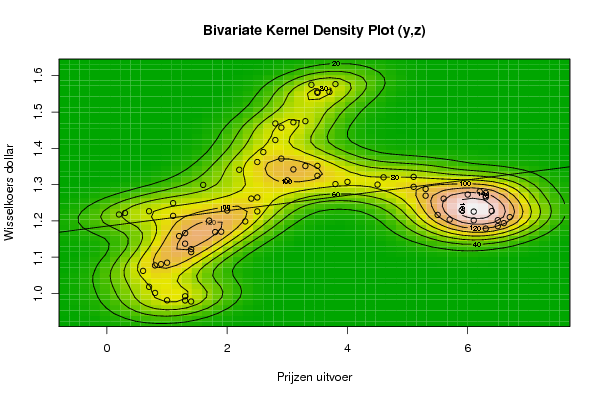
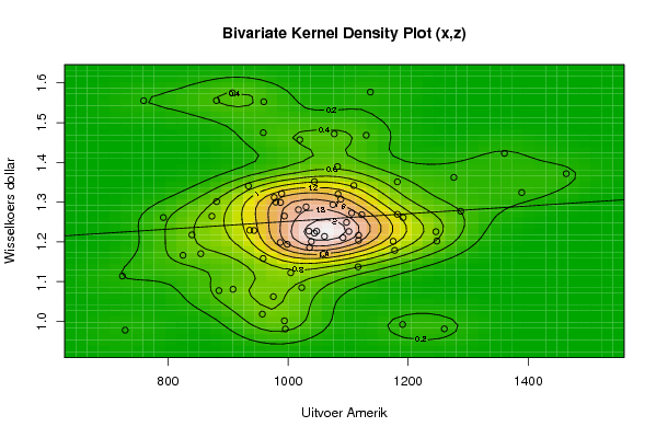
| Title produced by software | Trivariate Scatterplots | ||||||||||||||||||||
| Date of computation | Sun, 14 Dec 2008 05:48:40 -0700 | ||||||||||||||||||||
| Cite this page as follows | Statistical Computations at FreeStatistics.org, Office for Research Development and Education, URL https://freestatistics.org/blog/index.php?v=date/2008/Dec/14/t12292590781mycd9jxct77ima.htm/, Retrieved Wed, 15 May 2024 03:24:19 +0000 | ||||||||||||||||||||
| Statistical Computations at FreeStatistics.org, Office for Research Development and Education, URL https://freestatistics.org/blog/index.php?pk=33330, Retrieved Wed, 15 May 2024 03:24:19 +0000 | |||||||||||||||||||||
| QR Codes: | |||||||||||||||||||||
|
| |||||||||||||||||||||
| Original text written by user: | |||||||||||||||||||||
| IsPrivate? | No (this computation is public) | ||||||||||||||||||||
| User-defined keywords | |||||||||||||||||||||
| Estimated Impact | 180 | ||||||||||||||||||||
Tree of Dependent Computations | |||||||||||||||||||||
| Family? (F = Feedback message, R = changed R code, M = changed R Module, P = changed Parameters, D = changed Data) | |||||||||||||||||||||
| - [Kendall tau Rank Correlation] [Paper Kendall cor...] [2008-12-14 10:27:41] [9e54d1454d464f1bf9ee4a54d5d56945] - RMPD [Trivariate Scatterplots] [Paper: Trivariate...] [2008-12-14 12:48:40] [8da7502cfecb272886bc60b3f290b8b8] [Current] - [Trivariate Scatterplots] [] [2008-12-22 22:32:47] [187876c4ad94aebda16017e4a72ae602] | |||||||||||||||||||||
| Feedback Forum | |||||||||||||||||||||
Post a new message | |||||||||||||||||||||
Dataset | |||||||||||||||||||||
| Dataseries X: | |||||||||||||||||||||
1190,8 728,8 995,6 1260,3 994 957,3 975,6 884,9 908,4 1022,8 958,6 825,1 1116,6 724,2 1004,5 1058,9 854,7 943,4 792,4 873,2 1101,4 987,1 1038,8 1060,7 1047,7 840 1044 1097,4 987,5 934 977 881,1 1083,3 1074,7 1182,2 1117,5 1117,4 936,2 1246,3 1175,1 1177,7 1035,8 1091,6 998,7 1247,9 1034,7 1287,7 994,0 1122,8 1017,3 1106,0 1191,8 1030,1 989,4 979,6 1088,0 1389,2 1043,9 1182,1 1109,6 1463,3 1276,2 1082,4 1360,4 1130,2 1019,6 1077,0 958,8 959,6 907,2 880,8 759,6 1137,2 | |||||||||||||||||||||
| Dataseries Y: | |||||||||||||||||||||
1,3 1,4 1,3 1 0,8 0,7 0,6 0,8 0,9 1 1,2 1,3 1,3 1,4 1,4 1,8 1,9 2 2,4 2,5 2,5 2,3 1,7 1,1 0,7 0,2 0,3 1,1 1,6 2,2 3 3,8 4,6 5,1 5,3 5,5 5,7 5,9 6,1 6,1 6,3 6,5 6,7 6,6 6,5 6,4 6,3 6,3 6,3 6,2 6 5,6 5,3 5,1 4,5 4 3,5 3,5 3,3 3,1 2,9 2,5 2,6 2,8 2,8 2,9 3,1 3,3 3,5 3,4 3,5 3,7 3,8 | |||||||||||||||||||||
| Dataseries Z: | |||||||||||||||||||||
0,9922 0,9778 0,9808 0,9811 1,0014 1,0183 1,0622 1,0773 1,0807 1,0848 1,1582 1,1663 1,1372 1,1139 1,1222 1,1692 1,1702 1,2286 1,2613 1,2646 1,2262 1,1985 1,2007 1,2138 1,2266 1,2176 1,2218 1,249 1,2991 1,3408 1,3119 1,3014 1,3201 1,2938 1,2694 1,2165 1,2037 1,2292 1,2256 1,2015 1,1786 1,1856 1,2103 1,1938 1,202 1,2271 1,277 1,265 1,2684 1,2811 1,2727 1,2611 1,2881 1,3213 1,2999 1,3074 1,3242 1,3516 1,3511 1,3419 1,3716 1,3622 1,3896 1,4227 1,4684 1,457 1,4718 1,4748 1,5527 1,575 1,5557 1,5553 1,577 | |||||||||||||||||||||
Tables (Output of Computation) | |||||||||||||||||||||
| |||||||||||||||||||||
Figures (Output of Computation) | |||||||||||||||||||||
Input Parameters & R Code | |||||||||||||||||||||
| Parameters (Session): | |||||||||||||||||||||
| par1 = 50 ; par2 = 50 ; par3 = Y ; par4 = Y ; par5 = Uitvoer Amerik ; par6 = Prijzen uitvoer ; par7 = Wisselkoers dollar ; | |||||||||||||||||||||
| Parameters (R input): | |||||||||||||||||||||
| par1 = 50 ; par2 = 50 ; par3 = Y ; par4 = Y ; par5 = Uitvoer Amerik ; par6 = Prijzen uitvoer ; par7 = Wisselkoers dollar ; | |||||||||||||||||||||
| R code (references can be found in the software module): | |||||||||||||||||||||
x <- array(x,dim=c(length(x),1)) | |||||||||||||||||||||