Repository of Reproducible Computations

Free Statistics

of Irreproducible Research!

Author's title

Author

*The author of this computation has been verified*

R Software Module

rwasp_autocorrelation.wasp

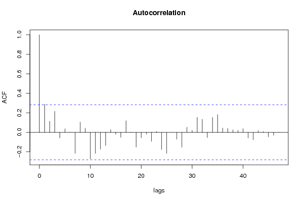
Title produced by software

(Partial) Autocorrelation Function

Date of computation

Fri, 12 Dec 2008 12:00:35 -0700

Cite this page as follows

Statistical Computations at FreeStatistics.org, Office for Research Development and Education, URL https://freestatistics.org/blog/index.php?v=date/2008/Dec/12/t1229108561egb3bjuj5a8siit.htm/, Retrieved Fri, 17 May 2024 13:30:39 +0000

Statistical Computations at FreeStatistics.org, Office for Research Development and Education, URL https://freestatistics.org/blog/index.php?pk=32869, Retrieved Fri, 17 May 2024 13:30:39 +0000

QR Codes:

Paste this QR Code to cite your computation.

Original text written by user:

IsPrivate?

No (this computation is public)

User-defined keywords

Estimated Impact

204

Family? (F = Feedback message, R = changed R code, M = changed R Module, P = changed Parameters, D = changed Data)

-     [Univariate Data Series] [Uitvoer.Nederland] [2008-12-03 15:11:10] [988ab43f527fc78aae41c84649095267]
-   P   [Univariate Data Series] [Export From Belgi...] [2008-12-03 15:52:29] [988ab43f527fc78aae41c84649095267]
- RMP     [Variance Reduction Matrix] [Variance Reductio...] [2008-12-03 15:56:08] [988ab43f527fc78aae41c84649095267]
- RMP       [(Partial) Autocorrelation Function] [Partial Autocorre...] [2008-12-03 16:40:39] [988ab43f527fc78aae41c84649095267]
-   PD        [(Partial) Autocorrelation Function] [arma model EU] [2008-12-11 17:29:01] [988ab43f527fc78aae41c84649095267]
-   PD          [(Partial) Autocorrelation Function] [Partial Autocorre...] [2008-12-12 18:59:02] [988ab43f527fc78aae41c84649095267]
-    D              [(Partial) Autocorrelation Function] [Partial Autocorre...] [2008-12-12 19:00:35] [5d823194959040fa9b19b8c8302177e6] [Current]

Feedback Forum

Post a new message

Dataseries X:

Download CSV

Histogram

Boxplots

Summary of computational transaction
Raw Input	view raw input (R code)
Raw Output	view raw output of R engine
Computing time	1 seconds
R Server	'George Udny Yule' @ 72.249.76.132

\begin{tabular}{lllllllll}
\hline
Summary of computational transaction \tabularnewline
Raw Input & view raw input (R code)  \tabularnewline
Raw Output & view raw output of R engine  \tabularnewline
Computing time & 1 seconds \tabularnewline
R Server & 'George Udny Yule' @ 72.249.76.132 \tabularnewline
\hline
\end{tabular}
%Source: https://freestatistics.org/blog/index.php?pk=32869&T=0

[TABLE]
[ROW][C]Summary of computational transaction[/C][/ROW]
[ROW][C]Raw Input[/C][C]view raw input (R code) [/C][/ROW]
[ROW][C]Raw Output[/C][C]view raw output of R engine [/C][/ROW]
[ROW][C]Computing time[/C][C]1 seconds[/C][/ROW]
[ROW][C]R Server[/C][C]'George Udny Yule' @ 72.249.76.132[/C][/ROW]
[/TABLE]
Source: https://freestatistics.org/blog/index.php?pk=32869&T=0

Globally Unique Identifier (entire table): ba.freestatistics.org/blog/index.php?pk=32869&T=0

As an alternative you can also use a QR Code:

The GUIDs for individual cells are displayed in the table below:

Summary of computational transaction
Raw Input	view raw input (R code)
Raw Output	view raw output of R engine
Computing time	1 seconds
R Server	'George Udny Yule' @ 72.249.76.132

Autocorrelation Function
Time lag k	ACF(k)	T-STAT	P-value
1	0.288979	2.0021	0.025471
2	0.114101	0.7905	0.216558
3	0.215396	1.4923	0.071082
4	-0.058024	-0.402	0.344732
5	0.036052	0.2498	0.401912
6	0.001031	0.0071	0.497165
7	-0.215813	-1.4952	0.070705
8	0.105466	0.7307	0.234261
9	0.041713	0.289	0.386913
10	-0.272899	-1.8907	0.032354
11	-0.216981	-1.5033	0.069658
12	-0.173635	-1.203	0.117442
13	-0.136104	-0.943	0.175212
14	0.02799	0.1939	0.423528
15	-0.019535	-0.1353	0.446453
16	-0.051026	-0.3535	0.362623
17	0.119108	0.8252	0.206668
18	-0.003443	-0.0239	0.490535
19	-0.151498	-1.0496	0.149577
20	-0.055167	-0.3822	0.351997
21	-0.019619	-0.1359	0.446225
22	-0.093067	-0.6448	0.261068
23	0.010406	0.0721	0.471412
24	-0.177307	-1.2284	0.112639
25	-0.216569	-1.5004	0.070025
26	-0.000487	-0.0034	0.498662
27	-0.070766	-0.4903	0.313084
28	-0.152431	-1.0561	0.148111
29	0.052219	0.3618	0.359552
30	0.020209	0.14	0.444617
31	0.154475	1.0702	0.144932
32	0.133559	0.9253	0.179713
33	-0.053811	-0.3728	0.355463
34	0.153585	1.0641	0.14631
35	0.181387	1.2567	0.107474
36	0.04383	0.3037	0.381347
37	0.040086	0.2777	0.391208
38	0.026681	0.1849	0.427062
39	0.020783	0.144	0.443056
40	0.038775	0.2686	0.394679
41	-0.058423	-0.4048	0.343723
42	-0.075671	-0.5243	0.301254
43	0.017537	0.1215	0.451902
44	0.008543	0.0592	0.476525
45	-0.046922	-0.3251	0.373264
46	-0.031189	-0.2161	0.414919
47	-0.001523	-0.0106	0.495812
48	NA	NA	NA

\begin{tabular}{lllllllll}
\hline
Autocorrelation Function \tabularnewline
Time lag k & ACF(k) & T-STAT & P-value \tabularnewline
1 & 0.288979 & 2.0021 & 0.025471 \tabularnewline
2 & 0.114101 & 0.7905 & 0.216558 \tabularnewline
3 & 0.215396 & 1.4923 & 0.071082 \tabularnewline
4 & -0.058024 & -0.402 & 0.344732 \tabularnewline
5 & 0.036052 & 0.2498 & 0.401912 \tabularnewline
6 & 0.001031 & 0.0071 & 0.497165 \tabularnewline
7 & -0.215813 & -1.4952 & 0.070705 \tabularnewline
8 & 0.105466 & 0.7307 & 0.234261 \tabularnewline
9 & 0.041713 & 0.289 & 0.386913 \tabularnewline
10 & -0.272899 & -1.8907 & 0.032354 \tabularnewline
11 & -0.216981 & -1.5033 & 0.069658 \tabularnewline
12 & -0.173635 & -1.203 & 0.117442 \tabularnewline
13 & -0.136104 & -0.943 & 0.175212 \tabularnewline
14 & 0.02799 & 0.1939 & 0.423528 \tabularnewline
15 & -0.019535 & -0.1353 & 0.446453 \tabularnewline
16 & -0.051026 & -0.3535 & 0.362623 \tabularnewline
17 & 0.119108 & 0.8252 & 0.206668 \tabularnewline
18 & -0.003443 & -0.0239 & 0.490535 \tabularnewline
19 & -0.151498 & -1.0496 & 0.149577 \tabularnewline
20 & -0.055167 & -0.3822 & 0.351997 \tabularnewline
21 & -0.019619 & -0.1359 & 0.446225 \tabularnewline
22 & -0.093067 & -0.6448 & 0.261068 \tabularnewline
23 & 0.010406 & 0.0721 & 0.471412 \tabularnewline
24 & -0.177307 & -1.2284 & 0.112639 \tabularnewline
25 & -0.216569 & -1.5004 & 0.070025 \tabularnewline
26 & -0.000487 & -0.0034 & 0.498662 \tabularnewline
27 & -0.070766 & -0.4903 & 0.313084 \tabularnewline
28 & -0.152431 & -1.0561 & 0.148111 \tabularnewline
29 & 0.052219 & 0.3618 & 0.359552 \tabularnewline
30 & 0.020209 & 0.14 & 0.444617 \tabularnewline
31 & 0.154475 & 1.0702 & 0.144932 \tabularnewline
32 & 0.133559 & 0.9253 & 0.179713 \tabularnewline
33 & -0.053811 & -0.3728 & 0.355463 \tabularnewline
34 & 0.153585 & 1.0641 & 0.14631 \tabularnewline
35 & 0.181387 & 1.2567 & 0.107474 \tabularnewline
36 & 0.04383 & 0.3037 & 0.381347 \tabularnewline
37 & 0.040086 & 0.2777 & 0.391208 \tabularnewline
38 & 0.026681 & 0.1849 & 0.427062 \tabularnewline
39 & 0.020783 & 0.144 & 0.443056 \tabularnewline
40 & 0.038775 & 0.2686 & 0.394679 \tabularnewline
41 & -0.058423 & -0.4048 & 0.343723 \tabularnewline
42 & -0.075671 & -0.5243 & 0.301254 \tabularnewline
43 & 0.017537 & 0.1215 & 0.451902 \tabularnewline
44 & 0.008543 & 0.0592 & 0.476525 \tabularnewline
45 & -0.046922 & -0.3251 & 0.373264 \tabularnewline
46 & -0.031189 & -0.2161 & 0.414919 \tabularnewline
47 & -0.001523 & -0.0106 & 0.495812 \tabularnewline
48 & NA & NA & NA \tabularnewline
\hline
\end{tabular}
%Source: https://freestatistics.org/blog/index.php?pk=32869&T=1

[TABLE]
[ROW][C]Autocorrelation Function[/C][/ROW]
[ROW][C]Time lag k[/C][C]ACF(k)[/C][C]T-STAT[/C][C]P-value[/C][/ROW]
[ROW][C]1[/C][C]0.288979[/C][C]2.0021[/C][C]0.025471[/C][/ROW]
[ROW][C]2[/C][C]0.114101[/C][C]0.7905[/C][C]0.216558[/C][/ROW]
[ROW][C]3[/C][C]0.215396[/C][C]1.4923[/C][C]0.071082[/C][/ROW]
[ROW][C]4[/C][C]-0.058024[/C][C]-0.402[/C][C]0.344732[/C][/ROW]
[ROW][C]5[/C][C]0.036052[/C][C]0.2498[/C][C]0.401912[/C][/ROW]
[ROW][C]6[/C][C]0.001031[/C][C]0.0071[/C][C]0.497165[/C][/ROW]
[ROW][C]7[/C][C]-0.215813[/C][C]-1.4952[/C][C]0.070705[/C][/ROW]
[ROW][C]8[/C][C]0.105466[/C][C]0.7307[/C][C]0.234261[/C][/ROW]
[ROW][C]9[/C][C]0.041713[/C][C]0.289[/C][C]0.386913[/C][/ROW]
[ROW][C]10[/C][C]-0.272899[/C][C]-1.8907[/C][C]0.032354[/C][/ROW]
[ROW][C]11[/C][C]-0.216981[/C][C]-1.5033[/C][C]0.069658[/C][/ROW]
[ROW][C]12[/C][C]-0.173635[/C][C]-1.203[/C][C]0.117442[/C][/ROW]
[ROW][C]13[/C][C]-0.136104[/C][C]-0.943[/C][C]0.175212[/C][/ROW]
[ROW][C]14[/C][C]0.02799[/C][C]0.1939[/C][C]0.423528[/C][/ROW]
[ROW][C]15[/C][C]-0.019535[/C][C]-0.1353[/C][C]0.446453[/C][/ROW]
[ROW][C]16[/C][C]-0.051026[/C][C]-0.3535[/C][C]0.362623[/C][/ROW]
[ROW][C]17[/C][C]0.119108[/C][C]0.8252[/C][C]0.206668[/C][/ROW]
[ROW][C]18[/C][C]-0.003443[/C][C]-0.0239[/C][C]0.490535[/C][/ROW]
[ROW][C]19[/C][C]-0.151498[/C][C]-1.0496[/C][C]0.149577[/C][/ROW]
[ROW][C]20[/C][C]-0.055167[/C][C]-0.3822[/C][C]0.351997[/C][/ROW]
[ROW][C]21[/C][C]-0.019619[/C][C]-0.1359[/C][C]0.446225[/C][/ROW]
[ROW][C]22[/C][C]-0.093067[/C][C]-0.6448[/C][C]0.261068[/C][/ROW]
[ROW][C]23[/C][C]0.010406[/C][C]0.0721[/C][C]0.471412[/C][/ROW]
[ROW][C]24[/C][C]-0.177307[/C][C]-1.2284[/C][C]0.112639[/C][/ROW]
[ROW][C]25[/C][C]-0.216569[/C][C]-1.5004[/C][C]0.070025[/C][/ROW]
[ROW][C]26[/C][C]-0.000487[/C][C]-0.0034[/C][C]0.498662[/C][/ROW]
[ROW][C]27[/C][C]-0.070766[/C][C]-0.4903[/C][C]0.313084[/C][/ROW]
[ROW][C]28[/C][C]-0.152431[/C][C]-1.0561[/C][C]0.148111[/C][/ROW]
[ROW][C]29[/C][C]0.052219[/C][C]0.3618[/C][C]0.359552[/C][/ROW]
[ROW][C]30[/C][C]0.020209[/C][C]0.14[/C][C]0.444617[/C][/ROW]
[ROW][C]31[/C][C]0.154475[/C][C]1.0702[/C][C]0.144932[/C][/ROW]
[ROW][C]32[/C][C]0.133559[/C][C]0.9253[/C][C]0.179713[/C][/ROW]
[ROW][C]33[/C][C]-0.053811[/C][C]-0.3728[/C][C]0.355463[/C][/ROW]
[ROW][C]34[/C][C]0.153585[/C][C]1.0641[/C][C]0.14631[/C][/ROW]
[ROW][C]35[/C][C]0.181387[/C][C]1.2567[/C][C]0.107474[/C][/ROW]
[ROW][C]36[/C][C]0.04383[/C][C]0.3037[/C][C]0.381347[/C][/ROW]
[ROW][C]37[/C][C]0.040086[/C][C]0.2777[/C][C]0.391208[/C][/ROW]
[ROW][C]38[/C][C]0.026681[/C][C]0.1849[/C][C]0.427062[/C][/ROW]
[ROW][C]39[/C][C]0.020783[/C][C]0.144[/C][C]0.443056[/C][/ROW]
[ROW][C]40[/C][C]0.038775[/C][C]0.2686[/C][C]0.394679[/C][/ROW]
[ROW][C]41[/C][C]-0.058423[/C][C]-0.4048[/C][C]0.343723[/C][/ROW]
[ROW][C]42[/C][C]-0.075671[/C][C]-0.5243[/C][C]0.301254[/C][/ROW]
[ROW][C]43[/C][C]0.017537[/C][C]0.1215[/C][C]0.451902[/C][/ROW]
[ROW][C]44[/C][C]0.008543[/C][C]0.0592[/C][C]0.476525[/C][/ROW]
[ROW][C]45[/C][C]-0.046922[/C][C]-0.3251[/C][C]0.373264[/C][/ROW]
[ROW][C]46[/C][C]-0.031189[/C][C]-0.2161[/C][C]0.414919[/C][/ROW]
[ROW][C]47[/C][C]-0.001523[/C][C]-0.0106[/C][C]0.495812[/C][/ROW]
[ROW][C]48[/C][C]NA[/C][C]NA[/C][C]NA[/C][/ROW]
[/TABLE]
Source: https://freestatistics.org/blog/index.php?pk=32869&T=1

Globally Unique Identifier (entire table): ba.freestatistics.org/blog/index.php?pk=32869&T=1

As an alternative you can also use a QR Code:

The GUIDs for individual cells are displayed in the table below:

Autocorrelation Function
Time lag k	ACF(k)	T-STAT	P-value
1	0.288979	2.0021	0.025471
2	0.114101	0.7905	0.216558
3	0.215396	1.4923	0.071082
4	-0.058024	-0.402	0.344732
5	0.036052	0.2498	0.401912
6	0.001031	0.0071	0.497165
7	-0.215813	-1.4952	0.070705
8	0.105466	0.7307	0.234261
9	0.041713	0.289	0.386913
10	-0.272899	-1.8907	0.032354
11	-0.216981	-1.5033	0.069658
12	-0.173635	-1.203	0.117442
13	-0.136104	-0.943	0.175212
14	0.02799	0.1939	0.423528
15	-0.019535	-0.1353	0.446453
16	-0.051026	-0.3535	0.362623
17	0.119108	0.8252	0.206668
18	-0.003443	-0.0239	0.490535
19	-0.151498	-1.0496	0.149577
20	-0.055167	-0.3822	0.351997
21	-0.019619	-0.1359	0.446225
22	-0.093067	-0.6448	0.261068
23	0.010406	0.0721	0.471412
24	-0.177307	-1.2284	0.112639
25	-0.216569	-1.5004	0.070025
26	-0.000487	-0.0034	0.498662
27	-0.070766	-0.4903	0.313084
28	-0.152431	-1.0561	0.148111
29	0.052219	0.3618	0.359552
30	0.020209	0.14	0.444617
31	0.154475	1.0702	0.144932
32	0.133559	0.9253	0.179713
33	-0.053811	-0.3728	0.355463
34	0.153585	1.0641	0.14631
35	0.181387	1.2567	0.107474
36	0.04383	0.3037	0.381347
37	0.040086	0.2777	0.391208
38	0.026681	0.1849	0.427062
39	0.020783	0.144	0.443056
40	0.038775	0.2686	0.394679
41	-0.058423	-0.4048	0.343723
42	-0.075671	-0.5243	0.301254
43	0.017537	0.1215	0.451902
44	0.008543	0.0592	0.476525
45	-0.046922	-0.3251	0.373264
46	-0.031189	-0.2161	0.414919
47	-0.001523	-0.0106	0.495812
48	NA	NA	NA

Partial Autocorrelation Function
Time lag k	PACF(k)	T-STAT	P-value
1	0.288979	2.0021	0.025471
2	0.03338	0.2313	0.409047
3	0.189932	1.3159	0.097231
4	-0.192043	-1.3305	0.094818
5	0.102252	0.7084	0.241055
6	-0.083683	-0.5798	0.282391
7	-0.167559	-1.1609	0.125715
8	0.224855	1.5578	0.06292
9	-0.03881	-0.2689	0.394586
10	-0.268605	-1.8609	0.034441
11	-0.21234	-1.4711	0.07389
12	0.027009	0.1871	0.426177
13	0.030988	0.2147	0.41546
14	0.0593	0.4108	0.341507
15	0.060206	0.4171	0.339226
16	-0.095436	-0.6612	0.255824
17	-0.00545	-0.0378	0.485019
18	-0.047141	-0.3266	0.372693
19	-0.085958	-0.5955	0.277141
20	-0.044577	-0.3088	0.37939
21	0.019473	0.1349	0.446622
22	-0.193043	-1.3374	0.093691
23	-0.030836	-0.2136	0.415868
24	-0.18058	-1.2511	0.108481
25	-0.141383	-0.9795	0.166114
26	0.043685	0.3027	0.381728
27	0.081989	0.568	0.286329
28	-0.14535	-1.007	0.159488
29	-0.037122	-0.2572	0.399066
30	2e-06	0	0.499994
31	0.109147	0.7562	0.226615
32	-0.077259	-0.5353	0.297469
33	-0.032642	-0.2261	0.411023
34	0.077733	0.5386	0.296343
35	-0.108636	-0.7527	0.227667
36	-0.021306	-0.1476	0.441635
37	-0.101229	-0.7013	0.243241
38	0.018958	0.1313	0.448025
39	-0.039411	-0.273	0.392994
40	-0.051822	-0.359	0.360573
41	0.026891	0.1863	0.426495
42	-0.016618	-0.1151	0.454411
43	-0.034173	-0.2368	0.406928
44	-0.070487	-0.4883	0.313764
45	0.064355	0.4459	0.328849
46	-0.049782	-0.3449	0.365837
47	-0.048708	-0.3375	0.36862
48	NA	NA	NA

\begin{tabular}{lllllllll}
\hline
Partial Autocorrelation Function \tabularnewline
Time lag k & PACF(k) & T-STAT & P-value \tabularnewline
1 & 0.288979 & 2.0021 & 0.025471 \tabularnewline
2 & 0.03338 & 0.2313 & 0.409047 \tabularnewline
3 & 0.189932 & 1.3159 & 0.097231 \tabularnewline
4 & -0.192043 & -1.3305 & 0.094818 \tabularnewline
5 & 0.102252 & 0.7084 & 0.241055 \tabularnewline
6 & -0.083683 & -0.5798 & 0.282391 \tabularnewline
7 & -0.167559 & -1.1609 & 0.125715 \tabularnewline
8 & 0.224855 & 1.5578 & 0.06292 \tabularnewline
9 & -0.03881 & -0.2689 & 0.394586 \tabularnewline
10 & -0.268605 & -1.8609 & 0.034441 \tabularnewline
11 & -0.21234 & -1.4711 & 0.07389 \tabularnewline
12 & 0.027009 & 0.1871 & 0.426177 \tabularnewline
13 & 0.030988 & 0.2147 & 0.41546 \tabularnewline
14 & 0.0593 & 0.4108 & 0.341507 \tabularnewline
15 & 0.060206 & 0.4171 & 0.339226 \tabularnewline
16 & -0.095436 & -0.6612 & 0.255824 \tabularnewline
17 & -0.00545 & -0.0378 & 0.485019 \tabularnewline
18 & -0.047141 & -0.3266 & 0.372693 \tabularnewline
19 & -0.085958 & -0.5955 & 0.277141 \tabularnewline
20 & -0.044577 & -0.3088 & 0.37939 \tabularnewline
21 & 0.019473 & 0.1349 & 0.446622 \tabularnewline
22 & -0.193043 & -1.3374 & 0.093691 \tabularnewline
23 & -0.030836 & -0.2136 & 0.415868 \tabularnewline
24 & -0.18058 & -1.2511 & 0.108481 \tabularnewline
25 & -0.141383 & -0.9795 & 0.166114 \tabularnewline
26 & 0.043685 & 0.3027 & 0.381728 \tabularnewline
27 & 0.081989 & 0.568 & 0.286329 \tabularnewline
28 & -0.14535 & -1.007 & 0.159488 \tabularnewline
29 & -0.037122 & -0.2572 & 0.399066 \tabularnewline
30 & 2e-06 & 0 & 0.499994 \tabularnewline
31 & 0.109147 & 0.7562 & 0.226615 \tabularnewline
32 & -0.077259 & -0.5353 & 0.297469 \tabularnewline
33 & -0.032642 & -0.2261 & 0.411023 \tabularnewline
34 & 0.077733 & 0.5386 & 0.296343 \tabularnewline
35 & -0.108636 & -0.7527 & 0.227667 \tabularnewline
36 & -0.021306 & -0.1476 & 0.441635 \tabularnewline
37 & -0.101229 & -0.7013 & 0.243241 \tabularnewline
38 & 0.018958 & 0.1313 & 0.448025 \tabularnewline
39 & -0.039411 & -0.273 & 0.392994 \tabularnewline
40 & -0.051822 & -0.359 & 0.360573 \tabularnewline
41 & 0.026891 & 0.1863 & 0.426495 \tabularnewline
42 & -0.016618 & -0.1151 & 0.454411 \tabularnewline
43 & -0.034173 & -0.2368 & 0.406928 \tabularnewline
44 & -0.070487 & -0.4883 & 0.313764 \tabularnewline
45 & 0.064355 & 0.4459 & 0.328849 \tabularnewline
46 & -0.049782 & -0.3449 & 0.365837 \tabularnewline
47 & -0.048708 & -0.3375 & 0.36862 \tabularnewline
48 & NA & NA & NA \tabularnewline
\hline
\end{tabular}
%Source: https://freestatistics.org/blog/index.php?pk=32869&T=2

[TABLE]
[ROW][C]Partial Autocorrelation Function[/C][/ROW]
[ROW][C]Time lag k[/C][C]PACF(k)[/C][C]T-STAT[/C][C]P-value[/C][/ROW]
[ROW][C]1[/C][C]0.288979[/C][C]2.0021[/C][C]0.025471[/C][/ROW]
[ROW][C]2[/C][C]0.03338[/C][C]0.2313[/C][C]0.409047[/C][/ROW]
[ROW][C]3[/C][C]0.189932[/C][C]1.3159[/C][C]0.097231[/C][/ROW]
[ROW][C]4[/C][C]-0.192043[/C][C]-1.3305[/C][C]0.094818[/C][/ROW]
[ROW][C]5[/C][C]0.102252[/C][C]0.7084[/C][C]0.241055[/C][/ROW]
[ROW][C]6[/C][C]-0.083683[/C][C]-0.5798[/C][C]0.282391[/C][/ROW]
[ROW][C]7[/C][C]-0.167559[/C][C]-1.1609[/C][C]0.125715[/C][/ROW]
[ROW][C]8[/C][C]0.224855[/C][C]1.5578[/C][C]0.06292[/C][/ROW]
[ROW][C]9[/C][C]-0.03881[/C][C]-0.2689[/C][C]0.394586[/C][/ROW]
[ROW][C]10[/C][C]-0.268605[/C][C]-1.8609[/C][C]0.034441[/C][/ROW]
[ROW][C]11[/C][C]-0.21234[/C][C]-1.4711[/C][C]0.07389[/C][/ROW]
[ROW][C]12[/C][C]0.027009[/C][C]0.1871[/C][C]0.426177[/C][/ROW]
[ROW][C]13[/C][C]0.030988[/C][C]0.2147[/C][C]0.41546[/C][/ROW]
[ROW][C]14[/C][C]0.0593[/C][C]0.4108[/C][C]0.341507[/C][/ROW]
[ROW][C]15[/C][C]0.060206[/C][C]0.4171[/C][C]0.339226[/C][/ROW]
[ROW][C]16[/C][C]-0.095436[/C][C]-0.6612[/C][C]0.255824[/C][/ROW]
[ROW][C]17[/C][C]-0.00545[/C][C]-0.0378[/C][C]0.485019[/C][/ROW]
[ROW][C]18[/C][C]-0.047141[/C][C]-0.3266[/C][C]0.372693[/C][/ROW]
[ROW][C]19[/C][C]-0.085958[/C][C]-0.5955[/C][C]0.277141[/C][/ROW]
[ROW][C]20[/C][C]-0.044577[/C][C]-0.3088[/C][C]0.37939[/C][/ROW]
[ROW][C]21[/C][C]0.019473[/C][C]0.1349[/C][C]0.446622[/C][/ROW]
[ROW][C]22[/C][C]-0.193043[/C][C]-1.3374[/C][C]0.093691[/C][/ROW]
[ROW][C]23[/C][C]-0.030836[/C][C]-0.2136[/C][C]0.415868[/C][/ROW]
[ROW][C]24[/C][C]-0.18058[/C][C]-1.2511[/C][C]0.108481[/C][/ROW]
[ROW][C]25[/C][C]-0.141383[/C][C]-0.9795[/C][C]0.166114[/C][/ROW]
[ROW][C]26[/C][C]0.043685[/C][C]0.3027[/C][C]0.381728[/C][/ROW]
[ROW][C]27[/C][C]0.081989[/C][C]0.568[/C][C]0.286329[/C][/ROW]
[ROW][C]28[/C][C]-0.14535[/C][C]-1.007[/C][C]0.159488[/C][/ROW]
[ROW][C]29[/C][C]-0.037122[/C][C]-0.2572[/C][C]0.399066[/C][/ROW]
[ROW][C]30[/C][C]2e-06[/C][C]0[/C][C]0.499994[/C][/ROW]
[ROW][C]31[/C][C]0.109147[/C][C]0.7562[/C][C]0.226615[/C][/ROW]
[ROW][C]32[/C][C]-0.077259[/C][C]-0.5353[/C][C]0.297469[/C][/ROW]
[ROW][C]33[/C][C]-0.032642[/C][C]-0.2261[/C][C]0.411023[/C][/ROW]
[ROW][C]34[/C][C]0.077733[/C][C]0.5386[/C][C]0.296343[/C][/ROW]
[ROW][C]35[/C][C]-0.108636[/C][C]-0.7527[/C][C]0.227667[/C][/ROW]
[ROW][C]36[/C][C]-0.021306[/C][C]-0.1476[/C][C]0.441635[/C][/ROW]
[ROW][C]37[/C][C]-0.101229[/C][C]-0.7013[/C][C]0.243241[/C][/ROW]
[ROW][C]38[/C][C]0.018958[/C][C]0.1313[/C][C]0.448025[/C][/ROW]
[ROW][C]39[/C][C]-0.039411[/C][C]-0.273[/C][C]0.392994[/C][/ROW]
[ROW][C]40[/C][C]-0.051822[/C][C]-0.359[/C][C]0.360573[/C][/ROW]
[ROW][C]41[/C][C]0.026891[/C][C]0.1863[/C][C]0.426495[/C][/ROW]
[ROW][C]42[/C][C]-0.016618[/C][C]-0.1151[/C][C]0.454411[/C][/ROW]
[ROW][C]43[/C][C]-0.034173[/C][C]-0.2368[/C][C]0.406928[/C][/ROW]
[ROW][C]44[/C][C]-0.070487[/C][C]-0.4883[/C][C]0.313764[/C][/ROW]
[ROW][C]45[/C][C]0.064355[/C][C]0.4459[/C][C]0.328849[/C][/ROW]
[ROW][C]46[/C][C]-0.049782[/C][C]-0.3449[/C][C]0.365837[/C][/ROW]
[ROW][C]47[/C][C]-0.048708[/C][C]-0.3375[/C][C]0.36862[/C][/ROW]
[ROW][C]48[/C][C]NA[/C][C]NA[/C][C]NA[/C][/ROW]
[/TABLE]
Source: https://freestatistics.org/blog/index.php?pk=32869&T=2

Globally Unique Identifier (entire table): ba.freestatistics.org/blog/index.php?pk=32869&T=2

As an alternative you can also use a QR Code:

The GUIDs for individual cells are displayed in the table below:

Partial Autocorrelation Function
Time lag k	PACF(k)	T-STAT	P-value
1	0.288979	2.0021	0.025471
2	0.03338	0.2313	0.409047
3	0.189932	1.3159	0.097231
4	-0.192043	-1.3305	0.094818
5	0.102252	0.7084	0.241055
6	-0.083683	-0.5798	0.282391
7	-0.167559	-1.1609	0.125715
8	0.224855	1.5578	0.06292
9	-0.03881	-0.2689	0.394586
10	-0.268605	-1.8609	0.034441
11	-0.21234	-1.4711	0.07389
12	0.027009	0.1871	0.426177
13	0.030988	0.2147	0.41546
14	0.0593	0.4108	0.341507
15	0.060206	0.4171	0.339226
16	-0.095436	-0.6612	0.255824
17	-0.00545	-0.0378	0.485019
18	-0.047141	-0.3266	0.372693
19	-0.085958	-0.5955	0.277141
20	-0.044577	-0.3088	0.37939
21	0.019473	0.1349	0.446622
22	-0.193043	-1.3374	0.093691
23	-0.030836	-0.2136	0.415868
24	-0.18058	-1.2511	0.108481
25	-0.141383	-0.9795	0.166114
26	0.043685	0.3027	0.381728
27	0.081989	0.568	0.286329
28	-0.14535	-1.007	0.159488
29	-0.037122	-0.2572	0.399066
30	2e-06	0	0.499994
31	0.109147	0.7562	0.226615
32	-0.077259	-0.5353	0.297469
33	-0.032642	-0.2261	0.411023
34	0.077733	0.5386	0.296343
35	-0.108636	-0.7527	0.227667
36	-0.021306	-0.1476	0.441635
37	-0.101229	-0.7013	0.243241
38	0.018958	0.1313	0.448025
39	-0.039411	-0.273	0.392994
40	-0.051822	-0.359	0.360573
41	0.026891	0.1863	0.426495
42	-0.016618	-0.1151	0.454411
43	-0.034173	-0.2368	0.406928
44	-0.070487	-0.4883	0.313764
45	0.064355	0.4459	0.328849
46	-0.049782	-0.3449	0.365837
47	-0.048708	-0.3375	0.36862
48	NA	NA	NA

Figure 1

PNG link

Postscript link

PDF link

Figure 2

PNG link

Postscript link

PDF link

Parameters (Session):

par1 = 12 ;

Parameters (R input):

par1 = 48 ; par2 = 1 ; par3 = 0 ; par4 = 1 ; par5 = 12 ;

R code (references can be found in the software module):

if (par1 == 'Default') {
par1 = 10*log10(length(x))
} else {
par1 <- as.numeric(par1)
}
par2 <- as.numeric(par2)
par3 <- as.numeric(par3)
par4 <- as.numeric(par4)
par5 <- as.numeric(par5)
if (par2 == 0) {
x <- log(x)
} else {
x <- (x ^ par2 - 1) / par2
}
if (par3 > 0) x <- diff(x,lag=1,difference=par3)
if (par4 > 0) x <- diff(x,lag=par5,difference=par4)
bitmap(file='pic1.png')
racf <- acf(x,par1,main='Autocorrelation',xlab='lags',ylab='ACF')
dev.off()
bitmap(file='pic2.png')
rpacf <- pacf(x,par1,main='Partial Autocorrelation',xlab='lags',ylab='PACF')
dev.off()
(myacf <- c(racf$acf))
(mypacf <- c(rpacf$acf))
lengthx <- length(x)
sqrtn <- sqrt(lengthx)
load(file='createtable')
a<-table.start()
a<-table.row.start(a)
a<-table.element(a,'Autocorrelation Function',4,TRUE)
a<-table.row.end(a)
a<-table.row.start(a)
a<-table.element(a,'Time lag k',header=TRUE)
a<-table.element(a,hyperlink('basics.htm','ACF(k)','click here for more information about the Autocorrelation Function'),header=TRUE)
a<-table.element(a,'T-STAT',header=TRUE)
a<-table.element(a,'P-value',header=TRUE)
a<-table.row.end(a)
for (i in 2:(par1+1)) {
a<-table.row.start(a)
a<-table.element(a,i-1,header=TRUE)
a<-table.element(a,round(myacf[i],6))
mytstat <- myacf[i]*sqrtn
a<-table.element(a,round(mytstat,4))
a<-table.element(a,round(1-pt(abs(mytstat),lengthx),6))
a<-table.row.end(a)
}
a<-table.end(a)
table.save(a,file='mytable.tab')
a<-table.start()
a<-table.row.start(a)
a<-table.element(a,'Partial Autocorrelation Function',4,TRUE)
a<-table.row.end(a)
a<-table.row.start(a)
a<-table.element(a,'Time lag k',header=TRUE)
a<-table.element(a,hyperlink('basics.htm','PACF(k)','click here for more information about the Partial Autocorrelation Function'),header=TRUE)
a<-table.element(a,'T-STAT',header=TRUE)
a<-table.element(a,'P-value',header=TRUE)
a<-table.row.end(a)
for (i in 1:par1) {
a<-table.row.start(a)
a<-table.element(a,i,header=TRUE)
a<-table.element(a,round(mypacf[i],6))
mytstat <- mypacf[i]*sqrtn
a<-table.element(a,round(mytstat,4))
a<-table.element(a,round(1-pt(abs(mytstat),lengthx),6))
a<-table.row.end(a)
}
a<-table.end(a)
table.save(a,file='mytable1.tab')

Free Statistics

Description of Statistical Computation

Tree of Dependent Computations

Dataset

Tables (Output of Computation)

Figures (Output of Computation)

Input Parameters & R Code