Repository of Reproducible Computations

Free Statistics

of Irreproducible Research!

Author's title

Author

*The author of this computation has been verified*

R Software Module

rwasp_arimaforecasting.wasp

Title produced by software

ARIMA Forecasting

Date of computation

Fri, 12 Dec 2008 10:26:53 -0700

Cite this page as follows

Statistical Computations at FreeStatistics.org, Office for Research Development and Education, URL https://freestatistics.org/blog/index.php?v=date/2008/Dec/12/t12291032362r6izgk4kvi9pac.htm/, Retrieved Mon, 20 May 2024 22:58:08 +0000

Statistical Computations at FreeStatistics.org, Office for Research Development and Education, URL https://freestatistics.org/blog/index.php?pk=32863, Retrieved Mon, 20 May 2024 22:58:08 +0000

QR Codes:

Paste this QR Code to cite your computation.

Original text written by user:

IsPrivate?

No (this computation is public)

User-defined keywords

Estimated Impact

203

Family? (F = Feedback message, R = changed R code, M = changed R Module, P = changed Parameters, D = changed Data)

-     [Univariate Data Series] [Run sequence plot...] [2008-12-02 21:55:47] [ed2ba3b6182103c15c0ab511ae4e6284]
- RMP   [Variance Reduction Matrix] [Variance reductio...] [2008-12-12 09:38:10] [ed2ba3b6182103c15c0ab511ae4e6284]
- RM      [Standard Deviation-Mean Plot] [Standard deviatio...] [2008-12-12 09:46:43] [ed2ba3b6182103c15c0ab511ae4e6284]
- RMP       [(Partial) Autocorrelation Function] [(P)ACF tabaksprod...] [2008-12-12 10:09:30] [ed2ba3b6182103c15c0ab511ae4e6284]
- RMP         [Spectral Analysis] [Spectrale analyse...] [2008-12-12 10:30:46] [ed2ba3b6182103c15c0ab511ae4e6284]
-               [Spectral Analysis] [Spectrale analyse...] [2008-12-12 11:05:23] [ed2ba3b6182103c15c0ab511ae4e6284]
- RMP             [ARIMA Backward Selection] [ARIMA backward se...] [2008-12-12 12:52:16] [ed2ba3b6182103c15c0ab511ae4e6284]
- RMPD                [ARIMA Forecasting] [] [2008-12-12 17:26:53] [19ef54504342c1b076371d395a2ab19f] [Current]

Feedback Forum

Post a new message

Dataseries X:

Download CSV

Histogram

Boxplots

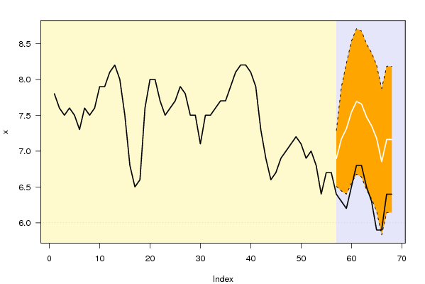
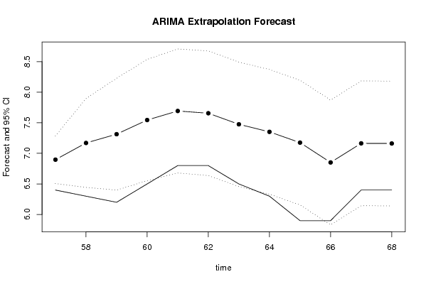
7.8
7.6
7.5
7.6
7.5
7.3
7.6
7.5
7.6
7.9
7.9
8.1
8.2
8.0
7.5
6.8
6.5
6.6
7.6
8.0
8.0
7.7
7.5
7.6
7.7
7.9
7.8
7.5
7.5
7.1
7.5
7.5
7.6
7.7
7.7
7.9
8.1
8.2
8.2
8.1
7.9
7.3
6.9
6.6
6.7
6.9
7.0
7.1
7.2
7.1
6.9
7.0
6.8
6.4
6.7
6.7
6.4
6.3
6.2
6.5
6.8
6.8
6.5
6.3
5.9
5.9
6.4
6.4

Summary of computational transaction
Raw Input	view raw input (R code)
Raw Output	view raw output of R engine
Computing time	1 seconds
R Server	'George Udny Yule' @ 72.249.76.132

\begin{tabular}{lllllllll}
\hline
Summary of computational transaction \tabularnewline
Raw Input & view raw input (R code)  \tabularnewline
Raw Output & view raw output of R engine  \tabularnewline
Computing time & 1 seconds \tabularnewline
R Server & 'George Udny Yule' @ 72.249.76.132 \tabularnewline
\hline
\end{tabular}
%Source: https://freestatistics.org/blog/index.php?pk=32863&T=0

[TABLE]
[ROW][C]Summary of computational transaction[/C][/ROW]
[ROW][C]Raw Input[/C][C]view raw input (R code) [/C][/ROW]
[ROW][C]Raw Output[/C][C]view raw output of R engine [/C][/ROW]
[ROW][C]Computing time[/C][C]1 seconds[/C][/ROW]
[ROW][C]R Server[/C][C]'George Udny Yule' @ 72.249.76.132[/C][/ROW]
[/TABLE]
Source: https://freestatistics.org/blog/index.php?pk=32863&T=0

Globally Unique Identifier (entire table): ba.freestatistics.org/blog/index.php?pk=32863&T=0

As an alternative you can also use a QR Code:

The GUIDs for individual cells are displayed in the table below:

Summary of computational transaction
Raw Input	view raw input (R code)
Raw Output	view raw output of R engine
Computing time	1 seconds
R Server	'George Udny Yule' @ 72.249.76.132

Univariate ARIMA Extrapolation Forecast
time	Y[t]	F[t]	95% LB	95% UB	p-value(H0: Y[t] = F[t])	P(F[t]>Y[t-1])	P(F[t]>Y[t-s])	P(F[t]>Y[56])
44	6.6	-	-	-	-	-	-	-
45	6.7	-	-	-	-	-	-	-
46	6.9	-	-	-	-	-	-	-
47	7	-	-	-	-	-	-	-
48	7.1	-	-	-	-	-	-	-
49	7.2	-	-	-	-	-	-	-
50	7.1	-	-	-	-	-	-	-
51	6.9	-	-	-	-	-	-	-
52	7	-	-	-	-	-	-	-
53	6.8	-	-	-	-	-	-	-
54	6.4	-	-	-	-	-	-	-
55	6.7	-	-	-	-	-	-	-
56	6.7	-	-	-	-	-	-	-
57	6.4	6.8968	6.5072	7.2863	0.0062	0.8389	0.8389	0.8389
58	6.3	7.1696	6.4436	7.8956	0.0094	0.9811	0.7666	0.8975
59	6.2	7.3134	6.3994	8.2274	0.0085	0.9851	0.7492	0.9058
60	6.5	7.5447	6.5534	8.5359	0.0194	0.9961	0.8104	0.9526
61	6.8	7.6926	6.6787	8.7066	0.0422	0.9894	0.8295	0.9725
62	6.8	7.6559	6.6379	8.6738	0.0497	0.9503	0.8577	0.9671
63	6.5	7.4751	6.4571	8.4931	0.0302	0.9032	0.8659	0.9322
64	6.3	7.3514	6.333	8.3698	0.0215	0.9493	0.7506	0.895
65	5.9	7.1756	6.1564	8.1947	0.0071	0.9539	0.7649	0.8198
66	5.9	6.8514	5.8317	7.8712	0.0337	0.9663	0.8072	0.6145
67	6.4	7.1635	6.1435	8.1835	0.0712	0.9924	0.8135	0.8135
68	6.4	7.1612	6.1413	8.1812	0.0718	0.9282	0.8123	0.8123

\begin{tabular}{lllllllll}
\hline
Univariate ARIMA Extrapolation Forecast \tabularnewline
time & Y[t] & F[t] & 95% LB & 95% UB & p-value(H0: Y[t] = F[t]) & P(F[t]>Y[t-1]) & P(F[t]>Y[t-s]) & P(F[t]>Y[56]) \tabularnewline
44 & 6.6 & - & - & - & - & - & - & - \tabularnewline
45 & 6.7 & - & - & - & - & - & - & - \tabularnewline
46 & 6.9 & - & - & - & - & - & - & - \tabularnewline
47 & 7 & - & - & - & - & - & - & - \tabularnewline
48 & 7.1 & - & - & - & - & - & - & - \tabularnewline
49 & 7.2 & - & - & - & - & - & - & - \tabularnewline
50 & 7.1 & - & - & - & - & - & - & - \tabularnewline
51 & 6.9 & - & - & - & - & - & - & - \tabularnewline
52 & 7 & - & - & - & - & - & - & - \tabularnewline
53 & 6.8 & - & - & - & - & - & - & - \tabularnewline
54 & 6.4 & - & - & - & - & - & - & - \tabularnewline
55 & 6.7 & - & - & - & - & - & - & - \tabularnewline
56 & 6.7 & - & - & - & - & - & - & - \tabularnewline
57 & 6.4 & 6.8968 & 6.5072 & 7.2863 & 0.0062 & 0.8389 & 0.8389 & 0.8389 \tabularnewline
58 & 6.3 & 7.1696 & 6.4436 & 7.8956 & 0.0094 & 0.9811 & 0.7666 & 0.8975 \tabularnewline
59 & 6.2 & 7.3134 & 6.3994 & 8.2274 & 0.0085 & 0.9851 & 0.7492 & 0.9058 \tabularnewline
60 & 6.5 & 7.5447 & 6.5534 & 8.5359 & 0.0194 & 0.9961 & 0.8104 & 0.9526 \tabularnewline
61 & 6.8 & 7.6926 & 6.6787 & 8.7066 & 0.0422 & 0.9894 & 0.8295 & 0.9725 \tabularnewline
62 & 6.8 & 7.6559 & 6.6379 & 8.6738 & 0.0497 & 0.9503 & 0.8577 & 0.9671 \tabularnewline
63 & 6.5 & 7.4751 & 6.4571 & 8.4931 & 0.0302 & 0.9032 & 0.8659 & 0.9322 \tabularnewline
64 & 6.3 & 7.3514 & 6.333 & 8.3698 & 0.0215 & 0.9493 & 0.7506 & 0.895 \tabularnewline
65 & 5.9 & 7.1756 & 6.1564 & 8.1947 & 0.0071 & 0.9539 & 0.7649 & 0.8198 \tabularnewline
66 & 5.9 & 6.8514 & 5.8317 & 7.8712 & 0.0337 & 0.9663 & 0.8072 & 0.6145 \tabularnewline
67 & 6.4 & 7.1635 & 6.1435 & 8.1835 & 0.0712 & 0.9924 & 0.8135 & 0.8135 \tabularnewline
68 & 6.4 & 7.1612 & 6.1413 & 8.1812 & 0.0718 & 0.9282 & 0.8123 & 0.8123 \tabularnewline
\hline
\end{tabular}
%Source: https://freestatistics.org/blog/index.php?pk=32863&T=1

[TABLE]
[ROW][C]Univariate ARIMA Extrapolation Forecast[/C][/ROW]
[ROW][C]time[/C][C]Y[t][/C][C]F[t][/C][C]95% LB[/C][C]95% UB[/C][C]p-value(H0: Y[t] = F[t])[/C][C]P(F[t]>Y[t-1])[/C][C]P(F[t]>Y[t-s])[/C][C]P(F[t]>Y[56])[/C][/ROW]
[ROW][C]44[/C][C]6.6[/C][C]-[/C][C]-[/C][C]-[/C][C]-[/C][C]-[/C][C]-[/C][C]-[/C][/ROW]
[ROW][C]45[/C][C]6.7[/C][C]-[/C][C]-[/C][C]-[/C][C]-[/C][C]-[/C][C]-[/C][C]-[/C][/ROW]
[ROW][C]46[/C][C]6.9[/C][C]-[/C][C]-[/C][C]-[/C][C]-[/C][C]-[/C][C]-[/C][C]-[/C][/ROW]
[ROW][C]47[/C][C]7[/C][C]-[/C][C]-[/C][C]-[/C][C]-[/C][C]-[/C][C]-[/C][C]-[/C][/ROW]
[ROW][C]48[/C][C]7.1[/C][C]-[/C][C]-[/C][C]-[/C][C]-[/C][C]-[/C][C]-[/C][C]-[/C][/ROW]
[ROW][C]49[/C][C]7.2[/C][C]-[/C][C]-[/C][C]-[/C][C]-[/C][C]-[/C][C]-[/C][C]-[/C][/ROW]
[ROW][C]50[/C][C]7.1[/C][C]-[/C][C]-[/C][C]-[/C][C]-[/C][C]-[/C][C]-[/C][C]-[/C][/ROW]
[ROW][C]51[/C][C]6.9[/C][C]-[/C][C]-[/C][C]-[/C][C]-[/C][C]-[/C][C]-[/C][C]-[/C][/ROW]
[ROW][C]52[/C][C]7[/C][C]-[/C][C]-[/C][C]-[/C][C]-[/C][C]-[/C][C]-[/C][C]-[/C][/ROW]
[ROW][C]53[/C][C]6.8[/C][C]-[/C][C]-[/C][C]-[/C][C]-[/C][C]-[/C][C]-[/C][C]-[/C][/ROW]
[ROW][C]54[/C][C]6.4[/C][C]-[/C][C]-[/C][C]-[/C][C]-[/C][C]-[/C][C]-[/C][C]-[/C][/ROW]
[ROW][C]55[/C][C]6.7[/C][C]-[/C][C]-[/C][C]-[/C][C]-[/C][C]-[/C][C]-[/C][C]-[/C][/ROW]
[ROW][C]56[/C][C]6.7[/C][C]-[/C][C]-[/C][C]-[/C][C]-[/C][C]-[/C][C]-[/C][C]-[/C][/ROW]
[ROW][C]57[/C][C]6.4[/C][C]6.8968[/C][C]6.5072[/C][C]7.2863[/C][C]0.0062[/C][C]0.8389[/C][C]0.8389[/C][C]0.8389[/C][/ROW]
[ROW][C]58[/C][C]6.3[/C][C]7.1696[/C][C]6.4436[/C][C]7.8956[/C][C]0.0094[/C][C]0.9811[/C][C]0.7666[/C][C]0.8975[/C][/ROW]
[ROW][C]59[/C][C]6.2[/C][C]7.3134[/C][C]6.3994[/C][C]8.2274[/C][C]0.0085[/C][C]0.9851[/C][C]0.7492[/C][C]0.9058[/C][/ROW]
[ROW][C]60[/C][C]6.5[/C][C]7.5447[/C][C]6.5534[/C][C]8.5359[/C][C]0.0194[/C][C]0.9961[/C][C]0.8104[/C][C]0.9526[/C][/ROW]
[ROW][C]61[/C][C]6.8[/C][C]7.6926[/C][C]6.6787[/C][C]8.7066[/C][C]0.0422[/C][C]0.9894[/C][C]0.8295[/C][C]0.9725[/C][/ROW]
[ROW][C]62[/C][C]6.8[/C][C]7.6559[/C][C]6.6379[/C][C]8.6738[/C][C]0.0497[/C][C]0.9503[/C][C]0.8577[/C][C]0.9671[/C][/ROW]
[ROW][C]63[/C][C]6.5[/C][C]7.4751[/C][C]6.4571[/C][C]8.4931[/C][C]0.0302[/C][C]0.9032[/C][C]0.8659[/C][C]0.9322[/C][/ROW]
[ROW][C]64[/C][C]6.3[/C][C]7.3514[/C][C]6.333[/C][C]8.3698[/C][C]0.0215[/C][C]0.9493[/C][C]0.7506[/C][C]0.895[/C][/ROW]
[ROW][C]65[/C][C]5.9[/C][C]7.1756[/C][C]6.1564[/C][C]8.1947[/C][C]0.0071[/C][C]0.9539[/C][C]0.7649[/C][C]0.8198[/C][/ROW]
[ROW][C]66[/C][C]5.9[/C][C]6.8514[/C][C]5.8317[/C][C]7.8712[/C][C]0.0337[/C][C]0.9663[/C][C]0.8072[/C][C]0.6145[/C][/ROW]
[ROW][C]67[/C][C]6.4[/C][C]7.1635[/C][C]6.1435[/C][C]8.1835[/C][C]0.0712[/C][C]0.9924[/C][C]0.8135[/C][C]0.8135[/C][/ROW]
[ROW][C]68[/C][C]6.4[/C][C]7.1612[/C][C]6.1413[/C][C]8.1812[/C][C]0.0718[/C][C]0.9282[/C][C]0.8123[/C][C]0.8123[/C][/ROW]
[/TABLE]
Source: https://freestatistics.org/blog/index.php?pk=32863&T=1

Globally Unique Identifier (entire table): ba.freestatistics.org/blog/index.php?pk=32863&T=1

As an alternative you can also use a QR Code:

The GUIDs for individual cells are displayed in the table below:

Univariate ARIMA Extrapolation Forecast
time	Y[t]	F[t]	95% LB	95% UB	p-value(H0: Y[t] = F[t])	P(F[t]>Y[t-1])	P(F[t]>Y[t-s])	P(F[t]>Y[56])
44	6.6	-	-	-	-	-	-	-
45	6.7	-	-	-	-	-	-	-
46	6.9	-	-	-	-	-	-	-
47	7	-	-	-	-	-	-	-
48	7.1	-	-	-	-	-	-	-
49	7.2	-	-	-	-	-	-	-
50	7.1	-	-	-	-	-	-	-
51	6.9	-	-	-	-	-	-	-
52	7	-	-	-	-	-	-	-
53	6.8	-	-	-	-	-	-	-
54	6.4	-	-	-	-	-	-	-
55	6.7	-	-	-	-	-	-	-
56	6.7	-	-	-	-	-	-	-
57	6.4	6.8968	6.5072	7.2863	0.0062	0.8389	0.8389	0.8389
58	6.3	7.1696	6.4436	7.8956	0.0094	0.9811	0.7666	0.8975
59	6.2	7.3134	6.3994	8.2274	0.0085	0.9851	0.7492	0.9058
60	6.5	7.5447	6.5534	8.5359	0.0194	0.9961	0.8104	0.9526
61	6.8	7.6926	6.6787	8.7066	0.0422	0.9894	0.8295	0.9725
62	6.8	7.6559	6.6379	8.6738	0.0497	0.9503	0.8577	0.9671
63	6.5	7.4751	6.4571	8.4931	0.0302	0.9032	0.8659	0.9322
64	6.3	7.3514	6.333	8.3698	0.0215	0.9493	0.7506	0.895
65	5.9	7.1756	6.1564	8.1947	0.0071	0.9539	0.7649	0.8198
66	5.9	6.8514	5.8317	7.8712	0.0337	0.9663	0.8072	0.6145
67	6.4	7.1635	6.1435	8.1835	0.0712	0.9924	0.8135	0.8135
68	6.4	7.1612	6.1413	8.1812	0.0718	0.9282	0.8123	0.8123

Univariate ARIMA Extrapolation Forecast Performance
time	% S.E.	PE	MAPE	Sq.E	MSE	RMSE
57	0.0288	-0.072	0.006	0.2468	0.0206	0.1434
58	0.0517	-0.1213	0.0101	0.7562	0.063	0.251
59	0.0638	-0.1522	0.0127	1.2396	0.1033	0.3214
60	0.067	-0.1385	0.0115	1.0913	0.0909	0.3016
61	0.0672	-0.116	0.0097	0.7968	0.0664	0.2577
62	0.0678	-0.1118	0.0093	0.7325	0.061	0.2471
63	0.0695	-0.1304	0.0109	0.9508	0.0792	0.2815
64	0.0707	-0.143	0.0119	1.1054	0.0921	0.3035
65	0.0725	-0.1778	0.0148	1.6271	0.1356	0.3682
66	0.0759	-0.1389	0.0116	0.9052	0.0754	0.2747
67	0.0726	-0.1066	0.0089	0.583	0.0486	0.2204
68	0.0727	-0.1063	0.0089	0.5795	0.0483	0.2198

\begin{tabular}{lllllllll}
\hline
Univariate ARIMA Extrapolation Forecast Performance \tabularnewline
time & % S.E. & PE & MAPE & Sq.E & MSE & RMSE \tabularnewline
57 & 0.0288 & -0.072 & 0.006 & 0.2468 & 0.0206 & 0.1434 \tabularnewline
58 & 0.0517 & -0.1213 & 0.0101 & 0.7562 & 0.063 & 0.251 \tabularnewline
59 & 0.0638 & -0.1522 & 0.0127 & 1.2396 & 0.1033 & 0.3214 \tabularnewline
60 & 0.067 & -0.1385 & 0.0115 & 1.0913 & 0.0909 & 0.3016 \tabularnewline
61 & 0.0672 & -0.116 & 0.0097 & 0.7968 & 0.0664 & 0.2577 \tabularnewline
62 & 0.0678 & -0.1118 & 0.0093 & 0.7325 & 0.061 & 0.2471 \tabularnewline
63 & 0.0695 & -0.1304 & 0.0109 & 0.9508 & 0.0792 & 0.2815 \tabularnewline
64 & 0.0707 & -0.143 & 0.0119 & 1.1054 & 0.0921 & 0.3035 \tabularnewline
65 & 0.0725 & -0.1778 & 0.0148 & 1.6271 & 0.1356 & 0.3682 \tabularnewline
66 & 0.0759 & -0.1389 & 0.0116 & 0.9052 & 0.0754 & 0.2747 \tabularnewline
67 & 0.0726 & -0.1066 & 0.0089 & 0.583 & 0.0486 & 0.2204 \tabularnewline
68 & 0.0727 & -0.1063 & 0.0089 & 0.5795 & 0.0483 & 0.2198 \tabularnewline
\hline
\end{tabular}
%Source: https://freestatistics.org/blog/index.php?pk=32863&T=2

[TABLE]
[ROW][C]Univariate ARIMA Extrapolation Forecast Performance[/C][/ROW]
[ROW][C]time[/C][C]% S.E.[/C][C]PE[/C][C]MAPE[/C][C]Sq.E[/C][C]MSE[/C][C]RMSE[/C][/ROW]
[ROW][C]57[/C][C]0.0288[/C][C]-0.072[/C][C]0.006[/C][C]0.2468[/C][C]0.0206[/C][C]0.1434[/C][/ROW]
[ROW][C]58[/C][C]0.0517[/C][C]-0.1213[/C][C]0.0101[/C][C]0.7562[/C][C]0.063[/C][C]0.251[/C][/ROW]
[ROW][C]59[/C][C]0.0638[/C][C]-0.1522[/C][C]0.0127[/C][C]1.2396[/C][C]0.1033[/C][C]0.3214[/C][/ROW]
[ROW][C]60[/C][C]0.067[/C][C]-0.1385[/C][C]0.0115[/C][C]1.0913[/C][C]0.0909[/C][C]0.3016[/C][/ROW]
[ROW][C]61[/C][C]0.0672[/C][C]-0.116[/C][C]0.0097[/C][C]0.7968[/C][C]0.0664[/C][C]0.2577[/C][/ROW]
[ROW][C]62[/C][C]0.0678[/C][C]-0.1118[/C][C]0.0093[/C][C]0.7325[/C][C]0.061[/C][C]0.2471[/C][/ROW]
[ROW][C]63[/C][C]0.0695[/C][C]-0.1304[/C][C]0.0109[/C][C]0.9508[/C][C]0.0792[/C][C]0.2815[/C][/ROW]
[ROW][C]64[/C][C]0.0707[/C][C]-0.143[/C][C]0.0119[/C][C]1.1054[/C][C]0.0921[/C][C]0.3035[/C][/ROW]
[ROW][C]65[/C][C]0.0725[/C][C]-0.1778[/C][C]0.0148[/C][C]1.6271[/C][C]0.1356[/C][C]0.3682[/C][/ROW]
[ROW][C]66[/C][C]0.0759[/C][C]-0.1389[/C][C]0.0116[/C][C]0.9052[/C][C]0.0754[/C][C]0.2747[/C][/ROW]
[ROW][C]67[/C][C]0.0726[/C][C]-0.1066[/C][C]0.0089[/C][C]0.583[/C][C]0.0486[/C][C]0.2204[/C][/ROW]
[ROW][C]68[/C][C]0.0727[/C][C]-0.1063[/C][C]0.0089[/C][C]0.5795[/C][C]0.0483[/C][C]0.2198[/C][/ROW]
[/TABLE]
Source: https://freestatistics.org/blog/index.php?pk=32863&T=2

Globally Unique Identifier (entire table): ba.freestatistics.org/blog/index.php?pk=32863&T=2

As an alternative you can also use a QR Code:

The GUIDs for individual cells are displayed in the table below:

Univariate ARIMA Extrapolation Forecast Performance
time	% S.E.	PE	MAPE	Sq.E	MSE	RMSE
57	0.0288	-0.072	0.006	0.2468	0.0206	0.1434
58	0.0517	-0.1213	0.0101	0.7562	0.063	0.251
59	0.0638	-0.1522	0.0127	1.2396	0.1033	0.3214
60	0.067	-0.1385	0.0115	1.0913	0.0909	0.3016
61	0.0672	-0.116	0.0097	0.7968	0.0664	0.2577
62	0.0678	-0.1118	0.0093	0.7325	0.061	0.2471
63	0.0695	-0.1304	0.0109	0.9508	0.0792	0.2815
64	0.0707	-0.143	0.0119	1.1054	0.0921	0.3035
65	0.0725	-0.1778	0.0148	1.6271	0.1356	0.3682
66	0.0759	-0.1389	0.0116	0.9052	0.0754	0.2747
67	0.0726	-0.1066	0.0089	0.583	0.0486	0.2204
68	0.0727	-0.1063	0.0089	0.5795	0.0483	0.2198

Figure 1

PNG link

Postscript link

PDF link

Figure 2

PNG link

Postscript link

PDF link

Parameters (Session):

par1 = 12 ; par2 = 1 ; par3 = 0 ; par4 = 1 ; par5 = 12 ; par6 = 2 ; par7 = 1 ; par8 = 1 ; par9 = 1 ; par10 = FALSE ;

Parameters (R input):

par1 = 12 ; par2 = 1 ; par3 = 0 ; par4 = 1 ; par5 = 12 ; par6 = 2 ; par7 = 1 ; par8 = 1 ; par9 = 1 ; par10 = FALSE ;

R code (references can be found in the software module):

par1 <- as.numeric(par1) #cut off periods
par2 <- as.numeric(par2) #lambda
par3 <- as.numeric(par3) #degree of non-seasonal differencing
par4 <- as.numeric(par4) #degree of seasonal differencing
par5 <- as.numeric(par5) #seasonal period
par6 <- as.numeric(par6) #p
par7 <- as.numeric(par7) #q
par8 <- as.numeric(par8) #P
par9 <- as.numeric(par9) #Q
if (par10 == 'TRUE') par10 <- TRUE
if (par10 == 'FALSE') par10 <- FALSE
if (par2 == 0) x <- log(x)
if (par2 != 0) x <- x^par2
lx <- length(x)
first <- lx - 2*par1
nx <- lx - par1
nx1 <- nx + 1
fx <- lx - nx
if (fx < 1) {
fx <- par5
nx1 <- lx + fx - 1
first <- lx - 2*fx
}
first <- 1
if (fx < 3) fx <- round(lx/10,0)
(arima.out <- arima(x[1:nx], order=c(par6,par3,par7), seasonal=list(order=c(par8,par4,par9), period=par5), include.mean=par10, method='ML'))
(forecast <- predict(arima.out,fx))
(lb <- forecast$pred - 1.96 * forecast$se)
(ub <- forecast$pred + 1.96 * forecast$se)
if (par2 == 0) {
x <- exp(x)
forecast$pred <- exp(forecast$pred)
lb <- exp(lb)
ub <- exp(ub)
}
if (par2 != 0) {
x <- x^(1/par2)
forecast$pred <- forecast$pred^(1/par2)
lb <- lb^(1/par2)
ub <- ub^(1/par2)
}
if (par2 < 0) {
olb <- lb
lb <- ub
ub <- olb
}
(actandfor <- c(x[1:nx], forecast$pred))
(perc.se <- (ub-forecast$pred)/1.96/forecast$pred)
bitmap(file='test1.png')
opar <- par(mar=c(4,4,2,2),las=1)
ylim <- c( min(x[first:nx],lb), max(x[first:nx],ub))
plot(x,ylim=ylim,type='n',xlim=c(first,lx))
usr <- par('usr')
rect(usr[1],usr[3],nx+1,usr[4],border=NA,col='lemonchiffon')
rect(nx1,usr[3],usr[2],usr[4],border=NA,col='lavender')
abline(h= (-3:3)*2 , col ='gray', lty =3)
polygon( c(nx1:lx,lx:nx1), c(lb,rev(ub)), col = 'orange', lty=2,border=NA)
lines(nx1:lx, lb , lty=2)
lines(nx1:lx, ub , lty=2)
lines(x, lwd=2)
lines(nx1:lx, forecast$pred , lwd=2 , col ='white')
box()
par(opar)
dev.off()
prob.dec <- array(NA, dim=fx)
prob.sdec <- array(NA, dim=fx)
prob.ldec <- array(NA, dim=fx)
prob.pval <- array(NA, dim=fx)
perf.pe <- array(0, dim=fx)
perf.mape <- array(0, dim=fx)
perf.se <- array(0, dim=fx)
perf.mse <- array(0, dim=fx)
perf.rmse <- array(0, dim=fx)
for (i in 1:fx) {
locSD <- (ub[i] - forecast$pred[i]) / 1.96
perf.pe[i] = (x[nx+i] - forecast$pred[i]) / forecast$pred[i]
perf.mape[i] = perf.mape[i] + abs(perf.pe[i])
perf.se[i] = (x[nx+i] - forecast$pred[i])^2
perf.mse[i] = perf.mse[i] + perf.se[i]
prob.dec[i] = pnorm((x[nx+i-1] - forecast$pred[i]) / locSD)
prob.sdec[i] = pnorm((x[nx+i-par5] - forecast$pred[i]) / locSD)
prob.ldec[i] = pnorm((x[nx] - forecast$pred[i]) / locSD)
prob.pval[i] = pnorm(abs(x[nx+i] - forecast$pred[i]) / locSD)
}
perf.mape = perf.mape / fx
perf.mse = perf.mse / fx
perf.rmse = sqrt(perf.mse)
bitmap(file='test2.png')
plot(forecast$pred, pch=19, type='b',main='ARIMA Extrapolation Forecast', ylab='Forecast and 95% CI', xlab='time',ylim=c(min(lb),max(ub)))
dum <- forecast$pred
dum[1:12] <- x[(nx+1):lx]
lines(dum, lty=1)
lines(ub,lty=3)
lines(lb,lty=3)
dev.off()
load(file='createtable')
a<-table.start()
a<-table.row.start(a)
a<-table.element(a,'Univariate ARIMA Extrapolation Forecast',9,TRUE)
a<-table.row.end(a)
a<-table.row.start(a)
a<-table.element(a,'time',1,header=TRUE)
a<-table.element(a,'Y[t]',1,header=TRUE)
a<-table.element(a,'F[t]',1,header=TRUE)
a<-table.element(a,'95% LB',1,header=TRUE)
a<-table.element(a,'95% UB',1,header=TRUE)
a<-table.element(a,'p-value
(H0: Y[t] = F[t])',1,header=TRUE)
a<-table.element(a,'P(F[t]>Y[t-1])',1,header=TRUE)
a<-table.element(a,'P(F[t]>Y[t-s])',1,header=TRUE)
mylab <- paste('P(F[t]>Y[',nx,sep='')
mylab <- paste(mylab,'])',sep='')
a<-table.element(a,mylab,1,header=TRUE)
a<-table.row.end(a)
for (i in (nx-par5):nx) {
a<-table.row.start(a)
a<-table.element(a,i,header=TRUE)
a<-table.element(a,x[i])
a<-table.element(a,'-')
a<-table.element(a,'-')
a<-table.element(a,'-')
a<-table.element(a,'-')
a<-table.element(a,'-')
a<-table.element(a,'-')
a<-table.element(a,'-')
a<-table.row.end(a)
}
for (i in 1:fx) {
a<-table.row.start(a)
a<-table.element(a,nx+i,header=TRUE)
a<-table.element(a,round(x[nx+i],4))
a<-table.element(a,round(forecast$pred[i],4))
a<-table.element(a,round(lb[i],4))
a<-table.element(a,round(ub[i],4))
a<-table.element(a,round((1-prob.pval[i]),4))
a<-table.element(a,round((1-prob.dec[i]),4))
a<-table.element(a,round((1-prob.sdec[i]),4))
a<-table.element(a,round((1-prob.ldec[i]),4))
a<-table.row.end(a)
}
a<-table.end(a)
table.save(a,file='mytable.tab')
a<-table.start()
a<-table.row.start(a)
a<-table.element(a,'Univariate ARIMA Extrapolation Forecast Performance',7,TRUE)
a<-table.row.end(a)
a<-table.row.start(a)
a<-table.element(a,'time',1,header=TRUE)
a<-table.element(a,'% S.E.',1,header=TRUE)
a<-table.element(a,'PE',1,header=TRUE)
a<-table.element(a,'MAPE',1,header=TRUE)
a<-table.element(a,'Sq.E',1,header=TRUE)
a<-table.element(a,'MSE',1,header=TRUE)
a<-table.element(a,'RMSE',1,header=TRUE)
a<-table.row.end(a)
for (i in 1:fx) {
a<-table.row.start(a)
a<-table.element(a,nx+i,header=TRUE)
a<-table.element(a,round(perc.se[i],4))
a<-table.element(a,round(perf.pe[i],4))
a<-table.element(a,round(perf.mape[i],4))
a<-table.element(a,round(perf.se[i],4))
a<-table.element(a,round(perf.mse[i],4))
a<-table.element(a,round(perf.rmse[i],4))
a<-table.row.end(a)
}
a<-table.end(a)
table.save(a,file='mytable1.tab')

Free Statistics

Description of Statistical Computation

Tree of Dependent Computations

Dataset

Tables (Output of Computation)

Figures (Output of Computation)

Input Parameters & R Code