Repository of Reproducible Computations

Free Statistics

of Irreproducible Research!

Author's title

Author

*The author of this computation has been verified*

R Software Module

rwasp_autocorrelation.wasp

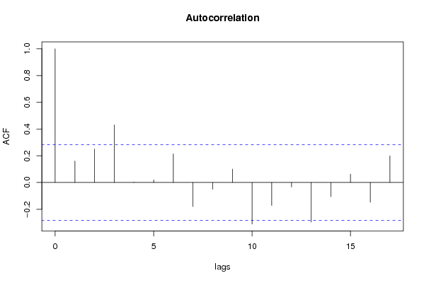
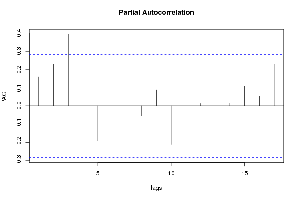
Title produced by software

(Partial) Autocorrelation Function

Date of computation

Fri, 12 Dec 2008 05:11:12 -0700

Cite this page as follows

Statistical Computations at FreeStatistics.org, Office for Research Development and Education, URL https://freestatistics.org/blog/index.php?v=date/2008/Dec/12/t1229083925glrqqxja2gobsdm.htm/, Retrieved Fri, 17 May 2024 16:29:48 +0000

Statistical Computations at FreeStatistics.org, Office for Research Development and Education, URL https://freestatistics.org/blog/index.php?pk=32603, Retrieved Fri, 17 May 2024 16:29:48 +0000

QR Codes:

Paste this QR Code to cite your computation.

Original text written by user:

IsPrivate?

No (this computation is public)

User-defined keywords

Estimated Impact

221

Family? (F = Feedback message, R = changed R code, M = changed R Module, P = changed Parameters, D = changed Data)

F     [Univariate Data Series] [Airline data] [2007-10-18 09:58:47] [42daae401fd3def69a25014f2252b4c2]
- R PD  [Univariate Data Series] [Tijdreeks 2 Buite...] [2008-12-11 16:25:30] [2d4aec5ed1856c4828162be37be304d9]
- RMP     [Central Tendency] [Central tendency ...] [2008-12-11 17:41:16] [2d4aec5ed1856c4828162be37be304d9]
- RMP       [Blocked Bootstrap Plot - Central Tendency] [Blocked Bootstrap...] [2008-12-12 08:14:08] [2d4aec5ed1856c4828162be37be304d9]
- RMP         [Tukey lambda PPCC Plot] [Tukey Lambda PPCC...] [2008-12-12 08:45:26] [2d4aec5ed1856c4828162be37be304d9]
- RMP           [Univariate Explorative Data Analysis] [Lag plot + ACF Ti...] [2008-12-12 08:54:04] [2d4aec5ed1856c4828162be37be304d9]
- RMP             [Variance Reduction Matrix] [VRM tijdreeks 2] [2008-12-12 10:58:24] [2d4aec5ed1856c4828162be37be304d9]
- RMP                 [(Partial) Autocorrelation Function] [P(ACF) Tijdreeks ...] [2008-12-12 12:11:12] [d7f41258beeebb8716e3f5d39f3cdc01] [Current]

Feedback Forum

Post a new message

Dataseries X:

Download CSV

Histogram

Boxplots

Summary of computational transaction
Raw Input	view raw input (R code)
Raw Output	view raw output of R engine
Computing time	2 seconds
R Server	'Gwilym Jenkins' @ 72.249.127.135

\begin{tabular}{lllllllll}
\hline
Summary of computational transaction \tabularnewline
Raw Input & view raw input (R code)  \tabularnewline
Raw Output & view raw output of R engine  \tabularnewline
Computing time & 2 seconds \tabularnewline
R Server & 'Gwilym Jenkins' @ 72.249.127.135 \tabularnewline
\hline
\end{tabular}
%Source: https://freestatistics.org/blog/index.php?pk=32603&T=0

[TABLE]
[ROW][C]Summary of computational transaction[/C][/ROW]
[ROW][C]Raw Input[/C][C]view raw input (R code) [/C][/ROW]
[ROW][C]Raw Output[/C][C]view raw output of R engine [/C][/ROW]
[ROW][C]Computing time[/C][C]2 seconds[/C][/ROW]
[ROW][C]R Server[/C][C]'Gwilym Jenkins' @ 72.249.127.135[/C][/ROW]
[/TABLE]
Source: https://freestatistics.org/blog/index.php?pk=32603&T=0

Globally Unique Identifier (entire table): ba.freestatistics.org/blog/index.php?pk=32603&T=0

As an alternative you can also use a QR Code:

The GUIDs for individual cells are displayed in the table below:

Summary of computational transaction
Raw Input	view raw input (R code)
Raw Output	view raw output of R engine
Computing time	2 seconds
R Server	'Gwilym Jenkins' @ 72.249.127.135

Autocorrelation Function
Time lag k	ACF(k)	T-STAT	P-value
1	0.160823	1.1142	0.135368
2	0.250663	1.7366	0.044432
3	0.430922	2.9855	0.002223
4	0.004201	0.0291	0.48845
5	0.019168	0.1328	0.447455
6	0.214298	1.4847	0.072081
7	-0.179766	-1.2455	0.109505
8	-0.050754	-0.3516	0.363326
9	0.101037	0.7	0.243651
10	-0.310381	-2.1504	0.018295
11	-0.17143	-1.1877	0.120398
12	-0.033674	-0.2333	0.408261
13	-0.296248	-2.0525	0.022799
14	-0.105688	-0.7322	0.233795
15	0.063056	0.4369	0.332084
16	-0.147309	-1.0206	0.156283
17	0.199064	1.3792	0.08712

\begin{tabular}{lllllllll}
\hline
Autocorrelation Function \tabularnewline
Time lag k & ACF(k) & T-STAT & P-value \tabularnewline
1 & 0.160823 & 1.1142 & 0.135368 \tabularnewline
2 & 0.250663 & 1.7366 & 0.044432 \tabularnewline
3 & 0.430922 & 2.9855 & 0.002223 \tabularnewline
4 & 0.004201 & 0.0291 & 0.48845 \tabularnewline
5 & 0.019168 & 0.1328 & 0.447455 \tabularnewline
6 & 0.214298 & 1.4847 & 0.072081 \tabularnewline
7 & -0.179766 & -1.2455 & 0.109505 \tabularnewline
8 & -0.050754 & -0.3516 & 0.363326 \tabularnewline
9 & 0.101037 & 0.7 & 0.243651 \tabularnewline
10 & -0.310381 & -2.1504 & 0.018295 \tabularnewline
11 & -0.17143 & -1.1877 & 0.120398 \tabularnewline
12 & -0.033674 & -0.2333 & 0.408261 \tabularnewline
13 & -0.296248 & -2.0525 & 0.022799 \tabularnewline
14 & -0.105688 & -0.7322 & 0.233795 \tabularnewline
15 & 0.063056 & 0.4369 & 0.332084 \tabularnewline
16 & -0.147309 & -1.0206 & 0.156283 \tabularnewline
17 & 0.199064 & 1.3792 & 0.08712 \tabularnewline
\hline
\end{tabular}
%Source: https://freestatistics.org/blog/index.php?pk=32603&T=1

[TABLE]
[ROW][C]Autocorrelation Function[/C][/ROW]
[ROW][C]Time lag k[/C][C]ACF(k)[/C][C]T-STAT[/C][C]P-value[/C][/ROW]
[ROW][C]1[/C][C]0.160823[/C][C]1.1142[/C][C]0.135368[/C][/ROW]
[ROW][C]2[/C][C]0.250663[/C][C]1.7366[/C][C]0.044432[/C][/ROW]
[ROW][C]3[/C][C]0.430922[/C][C]2.9855[/C][C]0.002223[/C][/ROW]
[ROW][C]4[/C][C]0.004201[/C][C]0.0291[/C][C]0.48845[/C][/ROW]
[ROW][C]5[/C][C]0.019168[/C][C]0.1328[/C][C]0.447455[/C][/ROW]
[ROW][C]6[/C][C]0.214298[/C][C]1.4847[/C][C]0.072081[/C][/ROW]
[ROW][C]7[/C][C]-0.179766[/C][C]-1.2455[/C][C]0.109505[/C][/ROW]
[ROW][C]8[/C][C]-0.050754[/C][C]-0.3516[/C][C]0.363326[/C][/ROW]
[ROW][C]9[/C][C]0.101037[/C][C]0.7[/C][C]0.243651[/C][/ROW]
[ROW][C]10[/C][C]-0.310381[/C][C]-2.1504[/C][C]0.018295[/C][/ROW]
[ROW][C]11[/C][C]-0.17143[/C][C]-1.1877[/C][C]0.120398[/C][/ROW]
[ROW][C]12[/C][C]-0.033674[/C][C]-0.2333[/C][C]0.408261[/C][/ROW]
[ROW][C]13[/C][C]-0.296248[/C][C]-2.0525[/C][C]0.022799[/C][/ROW]
[ROW][C]14[/C][C]-0.105688[/C][C]-0.7322[/C][C]0.233795[/C][/ROW]
[ROW][C]15[/C][C]0.063056[/C][C]0.4369[/C][C]0.332084[/C][/ROW]
[ROW][C]16[/C][C]-0.147309[/C][C]-1.0206[/C][C]0.156283[/C][/ROW]
[ROW][C]17[/C][C]0.199064[/C][C]1.3792[/C][C]0.08712[/C][/ROW]
[/TABLE]
Source: https://freestatistics.org/blog/index.php?pk=32603&T=1

Globally Unique Identifier (entire table): ba.freestatistics.org/blog/index.php?pk=32603&T=1

As an alternative you can also use a QR Code:

The GUIDs for individual cells are displayed in the table below:

Autocorrelation Function
Time lag k	ACF(k)	T-STAT	P-value
1	0.160823	1.1142	0.135368
2	0.250663	1.7366	0.044432
3	0.430922	2.9855	0.002223
4	0.004201	0.0291	0.48845
5	0.019168	0.1328	0.447455
6	0.214298	1.4847	0.072081
7	-0.179766	-1.2455	0.109505
8	-0.050754	-0.3516	0.363326
9	0.101037	0.7	0.243651
10	-0.310381	-2.1504	0.018295
11	-0.17143	-1.1877	0.120398
12	-0.033674	-0.2333	0.408261
13	-0.296248	-2.0525	0.022799
14	-0.105688	-0.7322	0.233795
15	0.063056	0.4369	0.332084
16	-0.147309	-1.0206	0.156283
17	0.199064	1.3792	0.08712

Partial Autocorrelation Function
Time lag k	PACF(k)	T-STAT	P-value
1	0.160823	1.1142	0.135368
2	0.230768	1.5988	0.058213
3	0.393381	2.7254	0.004468
4	-0.152526	-1.0567	0.147962
5	-0.193063	-1.3376	0.093669
6	0.119394	0.8272	0.206113
7	-0.141018	-0.977	0.166734
8	-0.056104	-0.3887	0.349608
9	0.089524	0.6202	0.269017
10	-0.211663	-1.4664	0.074525
11	-0.184465	-1.278	0.103695
12	0.012528	0.0868	0.465598
13	0.024183	0.1675	0.433823
14	0.015084	0.1045	0.458601
15	0.108945	0.7548	0.227031
16	0.0548	0.3797	0.352934
17	0.2313	1.6025	0.057804

\begin{tabular}{lllllllll}
\hline
Partial Autocorrelation Function \tabularnewline
Time lag k & PACF(k) & T-STAT & P-value \tabularnewline
1 & 0.160823 & 1.1142 & 0.135368 \tabularnewline
2 & 0.230768 & 1.5988 & 0.058213 \tabularnewline
3 & 0.393381 & 2.7254 & 0.004468 \tabularnewline
4 & -0.152526 & -1.0567 & 0.147962 \tabularnewline
5 & -0.193063 & -1.3376 & 0.093669 \tabularnewline
6 & 0.119394 & 0.8272 & 0.206113 \tabularnewline
7 & -0.141018 & -0.977 & 0.166734 \tabularnewline
8 & -0.056104 & -0.3887 & 0.349608 \tabularnewline
9 & 0.089524 & 0.6202 & 0.269017 \tabularnewline
10 & -0.211663 & -1.4664 & 0.074525 \tabularnewline
11 & -0.184465 & -1.278 & 0.103695 \tabularnewline
12 & 0.012528 & 0.0868 & 0.465598 \tabularnewline
13 & 0.024183 & 0.1675 & 0.433823 \tabularnewline
14 & 0.015084 & 0.1045 & 0.458601 \tabularnewline
15 & 0.108945 & 0.7548 & 0.227031 \tabularnewline
16 & 0.0548 & 0.3797 & 0.352934 \tabularnewline
17 & 0.2313 & 1.6025 & 0.057804 \tabularnewline
\hline
\end{tabular}
%Source: https://freestatistics.org/blog/index.php?pk=32603&T=2

[TABLE]
[ROW][C]Partial Autocorrelation Function[/C][/ROW]
[ROW][C]Time lag k[/C][C]PACF(k)[/C][C]T-STAT[/C][C]P-value[/C][/ROW]
[ROW][C]1[/C][C]0.160823[/C][C]1.1142[/C][C]0.135368[/C][/ROW]
[ROW][C]2[/C][C]0.230768[/C][C]1.5988[/C][C]0.058213[/C][/ROW]
[ROW][C]3[/C][C]0.393381[/C][C]2.7254[/C][C]0.004468[/C][/ROW]
[ROW][C]4[/C][C]-0.152526[/C][C]-1.0567[/C][C]0.147962[/C][/ROW]
[ROW][C]5[/C][C]-0.193063[/C][C]-1.3376[/C][C]0.093669[/C][/ROW]
[ROW][C]6[/C][C]0.119394[/C][C]0.8272[/C][C]0.206113[/C][/ROW]
[ROW][C]7[/C][C]-0.141018[/C][C]-0.977[/C][C]0.166734[/C][/ROW]
[ROW][C]8[/C][C]-0.056104[/C][C]-0.3887[/C][C]0.349608[/C][/ROW]
[ROW][C]9[/C][C]0.089524[/C][C]0.6202[/C][C]0.269017[/C][/ROW]
[ROW][C]10[/C][C]-0.211663[/C][C]-1.4664[/C][C]0.074525[/C][/ROW]
[ROW][C]11[/C][C]-0.184465[/C][C]-1.278[/C][C]0.103695[/C][/ROW]
[ROW][C]12[/C][C]0.012528[/C][C]0.0868[/C][C]0.465598[/C][/ROW]
[ROW][C]13[/C][C]0.024183[/C][C]0.1675[/C][C]0.433823[/C][/ROW]
[ROW][C]14[/C][C]0.015084[/C][C]0.1045[/C][C]0.458601[/C][/ROW]
[ROW][C]15[/C][C]0.108945[/C][C]0.7548[/C][C]0.227031[/C][/ROW]
[ROW][C]16[/C][C]0.0548[/C][C]0.3797[/C][C]0.352934[/C][/ROW]
[ROW][C]17[/C][C]0.2313[/C][C]1.6025[/C][C]0.057804[/C][/ROW]
[/TABLE]
Source: https://freestatistics.org/blog/index.php?pk=32603&T=2

Globally Unique Identifier (entire table): ba.freestatistics.org/blog/index.php?pk=32603&T=2

As an alternative you can also use a QR Code:

The GUIDs for individual cells are displayed in the table below:

Partial Autocorrelation Function
Time lag k	PACF(k)	T-STAT	P-value
1	0.160823	1.1142	0.135368
2	0.230768	1.5988	0.058213
3	0.393381	2.7254	0.004468
4	-0.152526	-1.0567	0.147962
5	-0.193063	-1.3376	0.093669
6	0.119394	0.8272	0.206113
7	-0.141018	-0.977	0.166734
8	-0.056104	-0.3887	0.349608
9	0.089524	0.6202	0.269017
10	-0.211663	-1.4664	0.074525
11	-0.184465	-1.278	0.103695
12	0.012528	0.0868	0.465598
13	0.024183	0.1675	0.433823
14	0.015084	0.1045	0.458601
15	0.108945	0.7548	0.227031
16	0.0548	0.3797	0.352934
17	0.2313	1.6025	0.057804

Figure 1

PNG link

Postscript link

PDF link

Figure 2

PNG link

Postscript link

PDF link

Parameters (Session):

par1 = Default ; par2 = 0.6 ; par3 = 0 ; par4 = 1 ; par5 = 12 ;

Parameters (R input):

par1 = Default ; par2 = 0.6 ; par3 = 0 ; par4 = 1 ; par5 = 12 ;

R code (references can be found in the software module):

if (par1 == 'Default') {
par1 = 10*log10(length(x))
} else {
par1 <- as.numeric(par1)
}
par2 <- as.numeric(par2)
par3 <- as.numeric(par3)
par4 <- as.numeric(par4)
par5 <- as.numeric(par5)
if (par2 == 0) {
x <- log(x)
} else {
x <- (x ^ par2 - 1) / par2
}
if (par3 > 0) x <- diff(x,lag=1,difference=par3)
if (par4 > 0) x <- diff(x,lag=par5,difference=par4)
bitmap(file='pic1.png')
racf <- acf(x,par1,main='Autocorrelation',xlab='lags',ylab='ACF')
dev.off()
bitmap(file='pic2.png')
rpacf <- pacf(x,par1,main='Partial Autocorrelation',xlab='lags',ylab='PACF')
dev.off()
(myacf <- c(racf$acf))
(mypacf <- c(rpacf$acf))
lengthx <- length(x)
sqrtn <- sqrt(lengthx)
load(file='createtable')
a<-table.start()
a<-table.row.start(a)
a<-table.element(a,'Autocorrelation Function',4,TRUE)
a<-table.row.end(a)
a<-table.row.start(a)
a<-table.element(a,'Time lag k',header=TRUE)
a<-table.element(a,hyperlink('basics.htm','ACF(k)','click here for more information about the Autocorrelation Function'),header=TRUE)
a<-table.element(a,'T-STAT',header=TRUE)
a<-table.element(a,'P-value',header=TRUE)
a<-table.row.end(a)
for (i in 2:(par1+1)) {
a<-table.row.start(a)
a<-table.element(a,i-1,header=TRUE)
a<-table.element(a,round(myacf[i],6))
mytstat <- myacf[i]*sqrtn
a<-table.element(a,round(mytstat,4))
a<-table.element(a,round(1-pt(abs(mytstat),lengthx),6))
a<-table.row.end(a)
}
a<-table.end(a)
table.save(a,file='mytable.tab')
a<-table.start()
a<-table.row.start(a)
a<-table.element(a,'Partial Autocorrelation Function',4,TRUE)
a<-table.row.end(a)
a<-table.row.start(a)
a<-table.element(a,'Time lag k',header=TRUE)
a<-table.element(a,hyperlink('basics.htm','PACF(k)','click here for more information about the Partial Autocorrelation Function'),header=TRUE)
a<-table.element(a,'T-STAT',header=TRUE)
a<-table.element(a,'P-value',header=TRUE)
a<-table.row.end(a)
for (i in 1:par1) {
a<-table.row.start(a)
a<-table.element(a,i,header=TRUE)
a<-table.element(a,round(mypacf[i],6))
mytstat <- mypacf[i]*sqrtn
a<-table.element(a,round(mytstat,4))
a<-table.element(a,round(1-pt(abs(mytstat),lengthx),6))
a<-table.row.end(a)
}
a<-table.end(a)
table.save(a,file='mytable1.tab')

Free Statistics

Description of Statistical Computation

Tree of Dependent Computations

Dataset

Tables (Output of Computation)

Figures (Output of Computation)

Input Parameters & R Code