Free Statistics
of Irreproducible Research!
Description of Statistical Computation | |||||||||||||||||||||||||||||||||||||||||||||||||||||||||||||||||||||||||||||||||||||||||||||||||||||||||||||||||||||||||||||||||
|---|---|---|---|---|---|---|---|---|---|---|---|---|---|---|---|---|---|---|---|---|---|---|---|---|---|---|---|---|---|---|---|---|---|---|---|---|---|---|---|---|---|---|---|---|---|---|---|---|---|---|---|---|---|---|---|---|---|---|---|---|---|---|---|---|---|---|---|---|---|---|---|---|---|---|---|---|---|---|---|---|---|---|---|---|---|---|---|---|---|---|---|---|---|---|---|---|---|---|---|---|---|---|---|---|---|---|---|---|---|---|---|---|---|---|---|---|---|---|---|---|---|---|---|---|---|---|---|---|---|
| Author's title | |||||||||||||||||||||||||||||||||||||||||||||||||||||||||||||||||||||||||||||||||||||||||||||||||||||||||||||||||||||||||||||||||
| Author | *The author of this computation has been verified* | ||||||||||||||||||||||||||||||||||||||||||||||||||||||||||||||||||||||||||||||||||||||||||||||||||||||||||||||||||||||||||||||||
| R Software Module | rwasp_smp.wasp | ||||||||||||||||||||||||||||||||||||||||||||||||||||||||||||||||||||||||||||||||||||||||||||||||||||||||||||||||||||||||||||||||
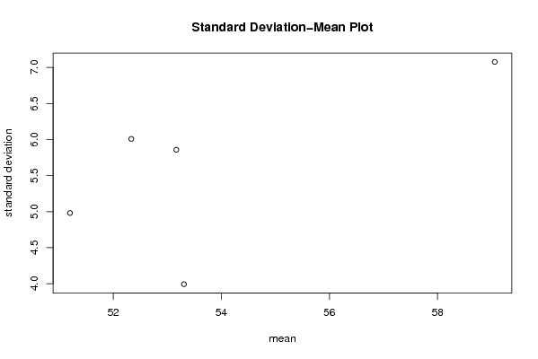
| Title produced by software | Standard Deviation-Mean Plot | ||||||||||||||||||||||||||||||||||||||||||||||||||||||||||||||||||||||||||||||||||||||||||||||||||||||||||||||||||||||||||||||||
| Date of computation | Fri, 12 Dec 2008 02:46:43 -0700 | ||||||||||||||||||||||||||||||||||||||||||||||||||||||||||||||||||||||||||||||||||||||||||||||||||||||||||||||||||||||||||||||||
| Cite this page as follows | Statistical Computations at FreeStatistics.org, Office for Research Development and Education, URL https://freestatistics.org/blog/index.php?v=date/2008/Dec/12/t12290752823pgyzjasd7aw4vt.htm/, Retrieved Tue, 21 May 2024 03:47:04 +0000 | ||||||||||||||||||||||||||||||||||||||||||||||||||||||||||||||||||||||||||||||||||||||||||||||||||||||||||||||||||||||||||||||||
| Statistical Computations at FreeStatistics.org, Office for Research Development and Education, URL https://freestatistics.org/blog/index.php?pk=32506, Retrieved Tue, 21 May 2024 03:47:04 +0000 | |||||||||||||||||||||||||||||||||||||||||||||||||||||||||||||||||||||||||||||||||||||||||||||||||||||||||||||||||||||||||||||||||
| QR Codes: | |||||||||||||||||||||||||||||||||||||||||||||||||||||||||||||||||||||||||||||||||||||||||||||||||||||||||||||||||||||||||||||||||
|
| |||||||||||||||||||||||||||||||||||||||||||||||||||||||||||||||||||||||||||||||||||||||||||||||||||||||||||||||||||||||||||||||||
| Original text written by user: | |||||||||||||||||||||||||||||||||||||||||||||||||||||||||||||||||||||||||||||||||||||||||||||||||||||||||||||||||||||||||||||||||
| IsPrivate? | No (this computation is public) | ||||||||||||||||||||||||||||||||||||||||||||||||||||||||||||||||||||||||||||||||||||||||||||||||||||||||||||||||||||||||||||||||
| User-defined keywords | |||||||||||||||||||||||||||||||||||||||||||||||||||||||||||||||||||||||||||||||||||||||||||||||||||||||||||||||||||||||||||||||||
| Estimated Impact | 263 | ||||||||||||||||||||||||||||||||||||||||||||||||||||||||||||||||||||||||||||||||||||||||||||||||||||||||||||||||||||||||||||||||
Tree of Dependent Computations | |||||||||||||||||||||||||||||||||||||||||||||||||||||||||||||||||||||||||||||||||||||||||||||||||||||||||||||||||||||||||||||||||
| Family? (F = Feedback message, R = changed R code, M = changed R Module, P = changed Parameters, D = changed Data) | |||||||||||||||||||||||||||||||||||||||||||||||||||||||||||||||||||||||||||||||||||||||||||||||||||||||||||||||||||||||||||||||||
| - [Univariate Data Series] [Run sequence plot...] [2008-12-02 21:55:47] [ed2ba3b6182103c15c0ab511ae4e6284] - RMP [Variance Reduction Matrix] [Variance reductio...] [2008-12-12 09:38:10] [ed2ba3b6182103c15c0ab511ae4e6284] - RM [Standard Deviation-Mean Plot] [Standard deviatio...] [2008-12-12 09:46:43] [a8228479d4547a92e2d3f176a5299609] [Current] - RMP [(Partial) Autocorrelation Function] [(P)ACF tabaksprod...] [2008-12-12 10:09:30] [ed2ba3b6182103c15c0ab511ae4e6284] - P [(Partial) Autocorrelation Function] [] [2008-12-12 10:26:36] [ed2ba3b6182103c15c0ab511ae4e6284] - [(Partial) Autocorrelation Function] [(P)ACF tabakspodu...] [2008-12-12 11:01:48] [ed2ba3b6182103c15c0ab511ae4e6284] - P [(Partial) Autocorrelation Function] [(P)ACF tabaksprod...] [2008-12-13 12:52:28] [ed2ba3b6182103c15c0ab511ae4e6284] - RMP [Spectral Analysis] [Spectrale analyse...] [2008-12-12 10:30:46] [ed2ba3b6182103c15c0ab511ae4e6284] - [Spectral Analysis] [Spectrale analyse...] [2008-12-12 11:05:23] [ed2ba3b6182103c15c0ab511ae4e6284] - RMP [ARIMA Backward Selection] [ARIMA backward se...] [2008-12-12 12:52:16] [ed2ba3b6182103c15c0ab511ae4e6284] - RMPD [ARIMA Forecasting] [] [2008-12-12 14:09:09] [a4ee3bef49b119f4bd2e925060c84f5e] - PD [ARIMA Backward Selection] [] [2008-12-12 14:08:29] [a4ee3bef49b119f4bd2e925060c84f5e] - RMP [(Partial) Autocorrelation Function] [] [2008-12-12 14:06:36] [a4ee3bef49b119f4bd2e925060c84f5e] - PD [ARIMA Backward Selection] [] [2008-12-12 17:29:27] [a4ee3bef49b119f4bd2e925060c84f5e] - RMPD [ARIMA Forecasting] [] [2008-12-12 17:26:53] [a4ee3bef49b119f4bd2e925060c84f5e] - RMP [ARIMA Backward Selection] [ARIMA blog] [2008-12-12 13:09:51] [ed2ba3b6182103c15c0ab511ae4e6284] - P [Spectral Analysis] [Spectrale analyse...] [2008-12-13 13:07:40] [ed2ba3b6182103c15c0ab511ae4e6284] | |||||||||||||||||||||||||||||||||||||||||||||||||||||||||||||||||||||||||||||||||||||||||||||||||||||||||||||||||||||||||||||||||
| Feedback Forum | |||||||||||||||||||||||||||||||||||||||||||||||||||||||||||||||||||||||||||||||||||||||||||||||||||||||||||||||||||||||||||||||||
Post a new message | |||||||||||||||||||||||||||||||||||||||||||||||||||||||||||||||||||||||||||||||||||||||||||||||||||||||||||||||||||||||||||||||||
Dataset | |||||||||||||||||||||||||||||||||||||||||||||||||||||||||||||||||||||||||||||||||||||||||||||||||||||||||||||||||||||||||||||||||
| Dataseries X: | |||||||||||||||||||||||||||||||||||||||||||||||||||||||||||||||||||||||||||||||||||||||||||||||||||||||||||||||||||||||||||||||||
44.9 48.1 52.3 48.9 52.6 60.3 50.5 41.6 56 51.4 52.9 54.9 43.9 51 51.9 54.3 50.3 57.2 48.8 41.1 58 63 53.8 54.7 55.5 56.1 69.6 69.4 57.2 68 53.3 47.9 60.8 61.7 57.8 51.4 50.5 48.1 58.7 54 56.1 60.4 51.2 50.7 56.4 53.3 52.6 47.7 49.5 48.5 55.3 49.8 57.4 64.6 53 41.5 55.9 58.4 53.5 50.6 58.5 | |||||||||||||||||||||||||||||||||||||||||||||||||||||||||||||||||||||||||||||||||||||||||||||||||||||||||||||||||||||||||||||||||
Tables (Output of Computation) | |||||||||||||||||||||||||||||||||||||||||||||||||||||||||||||||||||||||||||||||||||||||||||||||||||||||||||||||||||||||||||||||||
| |||||||||||||||||||||||||||||||||||||||||||||||||||||||||||||||||||||||||||||||||||||||||||||||||||||||||||||||||||||||||||||||||
Figures (Output of Computation) | |||||||||||||||||||||||||||||||||||||||||||||||||||||||||||||||||||||||||||||||||||||||||||||||||||||||||||||||||||||||||||||||||
Input Parameters & R Code | |||||||||||||||||||||||||||||||||||||||||||||||||||||||||||||||||||||||||||||||||||||||||||||||||||||||||||||||||||||||||||||||||
| Parameters (Session): | |||||||||||||||||||||||||||||||||||||||||||||||||||||||||||||||||||||||||||||||||||||||||||||||||||||||||||||||||||||||||||||||||
| par1 = 12 ; | |||||||||||||||||||||||||||||||||||||||||||||||||||||||||||||||||||||||||||||||||||||||||||||||||||||||||||||||||||||||||||||||||
| Parameters (R input): | |||||||||||||||||||||||||||||||||||||||||||||||||||||||||||||||||||||||||||||||||||||||||||||||||||||||||||||||||||||||||||||||||
| par1 = 12 ; | |||||||||||||||||||||||||||||||||||||||||||||||||||||||||||||||||||||||||||||||||||||||||||||||||||||||||||||||||||||||||||||||||
| R code (references can be found in the software module): | |||||||||||||||||||||||||||||||||||||||||||||||||||||||||||||||||||||||||||||||||||||||||||||||||||||||||||||||||||||||||||||||||
par1 <- as.numeric(par1) | |||||||||||||||||||||||||||||||||||||||||||||||||||||||||||||||||||||||||||||||||||||||||||||||||||||||||||||||||||||||||||||||||