Free Statistics
of Irreproducible Research!
Description of Statistical Computation | |||||||||||||||||||||||||||||||||||||||||||||||||||||
|---|---|---|---|---|---|---|---|---|---|---|---|---|---|---|---|---|---|---|---|---|---|---|---|---|---|---|---|---|---|---|---|---|---|---|---|---|---|---|---|---|---|---|---|---|---|---|---|---|---|---|---|---|---|
| Author's title | |||||||||||||||||||||||||||||||||||||||||||||||||||||
| Author | *The author of this computation has been verified* | ||||||||||||||||||||||||||||||||||||||||||||||||||||
| R Software Module | rwasp_edauni.wasp | ||||||||||||||||||||||||||||||||||||||||||||||||||||
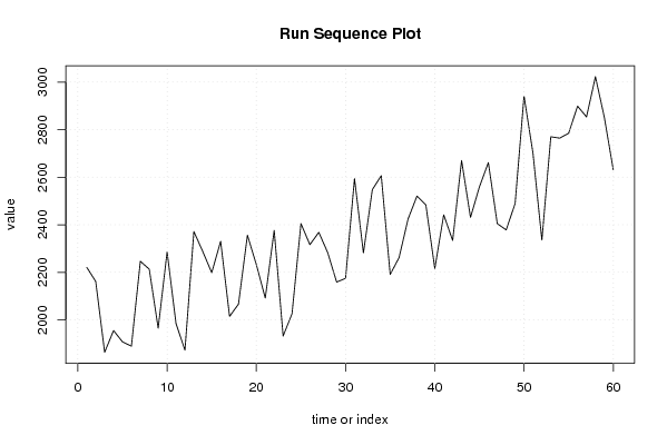
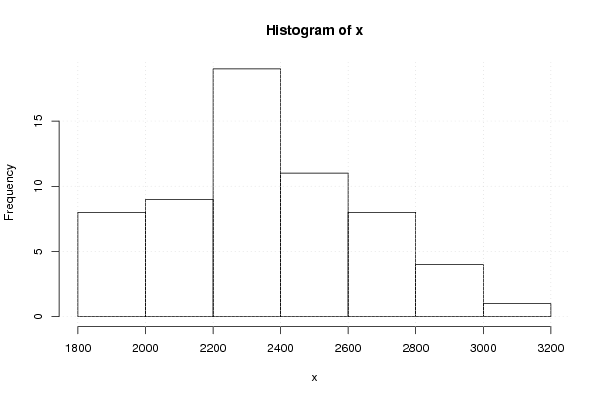
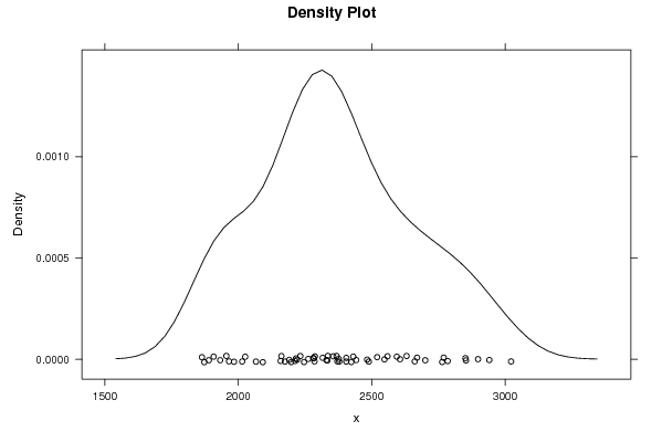
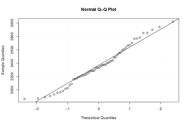
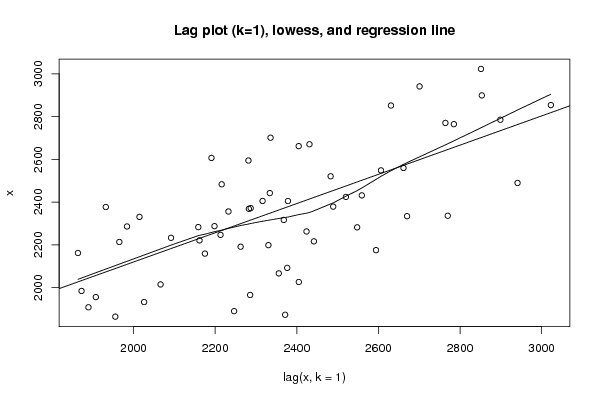
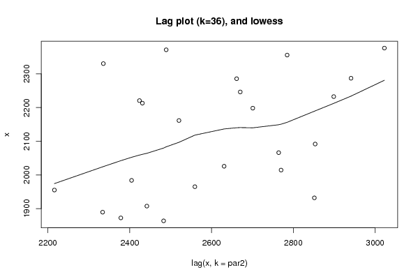
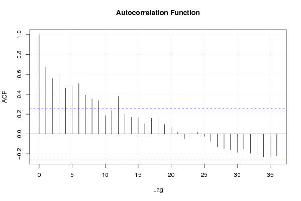
| Title produced by software | Univariate Explorative Data Analysis | ||||||||||||||||||||||||||||||||||||||||||||||||||||
| Date of computation | Fri, 12 Dec 2008 01:54:04 -0700 | ||||||||||||||||||||||||||||||||||||||||||||||||||||
| Cite this page as follows | Statistical Computations at FreeStatistics.org, Office for Research Development and Education, URL https://freestatistics.org/blog/index.php?v=date/2008/Dec/12/t1229072153k0gbtltetcu44aj.htm/, Retrieved Fri, 17 May 2024 13:41:47 +0000 | ||||||||||||||||||||||||||||||||||||||||||||||||||||
| Statistical Computations at FreeStatistics.org, Office for Research Development and Education, URL https://freestatistics.org/blog/index.php?pk=32489, Retrieved Fri, 17 May 2024 13:41:47 +0000 | |||||||||||||||||||||||||||||||||||||||||||||||||||||
| QR Codes: | |||||||||||||||||||||||||||||||||||||||||||||||||||||
|
| |||||||||||||||||||||||||||||||||||||||||||||||||||||
| Original text written by user: | |||||||||||||||||||||||||||||||||||||||||||||||||||||
| IsPrivate? | No (this computation is public) | ||||||||||||||||||||||||||||||||||||||||||||||||||||
| User-defined keywords | |||||||||||||||||||||||||||||||||||||||||||||||||||||
| Estimated Impact | 243 | ||||||||||||||||||||||||||||||||||||||||||||||||||||
Tree of Dependent Computations | |||||||||||||||||||||||||||||||||||||||||||||||||||||
| Family? (F = Feedback message, R = changed R code, M = changed R Module, P = changed Parameters, D = changed Data) | |||||||||||||||||||||||||||||||||||||||||||||||||||||
| F [Univariate Data Series] [Airline data] [2007-10-18 09:58:47] [42daae401fd3def69a25014f2252b4c2] - R PD [Univariate Data Series] [Tijdreeks 2 Buite...] [2008-12-11 16:25:30] [2d4aec5ed1856c4828162be37be304d9] - RMP [Central Tendency] [Central tendency ...] [2008-12-11 17:41:16] [2d4aec5ed1856c4828162be37be304d9] - RMP [Blocked Bootstrap Plot - Central Tendency] [Blocked Bootstrap...] [2008-12-12 08:14:08] [2d4aec5ed1856c4828162be37be304d9] - RMP [Tukey lambda PPCC Plot] [Tukey Lambda PPCC...] [2008-12-12 08:45:26] [2d4aec5ed1856c4828162be37be304d9] - RMP [Univariate Explorative Data Analysis] [Lag plot + ACF Ti...] [2008-12-12 08:54:04] [d7f41258beeebb8716e3f5d39f3cdc01] [Current] - RMP [Variance Reduction Matrix] [VRM tijdreeks 2] [2008-12-12 10:58:24] [2d4aec5ed1856c4828162be37be304d9] - RMP [Spectral Analysis] [Spectrum tijdreeks 2] [2008-12-12 11:59:54] [2d4aec5ed1856c4828162be37be304d9] - RMP [(Partial) Autocorrelation Function] [P(ACF) Tijdreeks ...] [2008-12-12 12:11:12] [2d4aec5ed1856c4828162be37be304d9] - RMP [(Partial) Autocorrelation Function] [P(ACF) Tijdreeks ...] [2008-12-12 12:17:09] [2d4aec5ed1856c4828162be37be304d9] - RMP [ARIMA Backward Selection] [ARIMA Backward Se...] [2008-12-12 12:29:19] [2d4aec5ed1856c4828162be37be304d9] - RMPD [Bivariate Kernel Density Estimation] [Bivariate Kernel ...] [2008-12-22 09:26:11] [2d4aec5ed1856c4828162be37be304d9] - RMPD [Kendall tau Correlation Matrix] [Kendall Tau Corre...] [2008-12-22 09:35:25] [2d4aec5ed1856c4828162be37be304d9] - RM D [Pearson Correlation] [Pearson correlati...] [2008-12-22 09:46:51] [2d4aec5ed1856c4828162be37be304d9] - RMP [Cross Correlation Function] [Cross Correlation...] [2008-12-22 10:31:31] [2d4aec5ed1856c4828162be37be304d9] - P [Cross Correlation Function] [Cross Correlation...] [2008-12-22 11:21:14] [2d4aec5ed1856c4828162be37be304d9] - RMP [ARIMA Forecasting] [Arima forecast (p...] [2008-12-22 15:10:16] [2d4aec5ed1856c4828162be37be304d9] - D [Variance Reduction Matrix] [VRM Xt] [2008-12-22 11:17:14] [2d4aec5ed1856c4828162be37be304d9] | |||||||||||||||||||||||||||||||||||||||||||||||||||||
| Feedback Forum | |||||||||||||||||||||||||||||||||||||||||||||||||||||
Post a new message | |||||||||||||||||||||||||||||||||||||||||||||||||||||
Dataset | |||||||||||||||||||||||||||||||||||||||||||||||||||||
| Dataseries X: | |||||||||||||||||||||||||||||||||||||||||||||||||||||
2220.6 2161.5 1863.6 1955.1 1907.4 1889.4 2246.3 2213 1965 2285.6 1983.8 1872.4 2371.4 2287 2198.2 2330.4 2014.4 2066.1 2355.8 2232.5 2091.7 2376.5 1931.9 2025.7 2404.9 2316.1 2368.1 2282.5 2158.6 2174.8 2594.1 2281.4 2547.9 2606.3 2190.8 2262.3 2423.8 2520.4 2482.9 2215.9 2441.9 2333.8 2670.2 2431 2559.3 2661.4 2404.6 2378.3 2489.2 2941 2700.9 2335.6 2770 2764.2 2784.9 2898.8 2853.4 3022.6 2851.4 2630.8 | |||||||||||||||||||||||||||||||||||||||||||||||||||||
Tables (Output of Computation) | |||||||||||||||||||||||||||||||||||||||||||||||||||||
| |||||||||||||||||||||||||||||||||||||||||||||||||||||
Figures (Output of Computation) | |||||||||||||||||||||||||||||||||||||||||||||||||||||
Input Parameters & R Code | |||||||||||||||||||||||||||||||||||||||||||||||||||||
| Parameters (Session): | |||||||||||||||||||||||||||||||||||||||||||||||||||||
| par1 = 0 ; par2 = 36 ; | |||||||||||||||||||||||||||||||||||||||||||||||||||||
| Parameters (R input): | |||||||||||||||||||||||||||||||||||||||||||||||||||||
| par1 = 0 ; par2 = 36 ; | |||||||||||||||||||||||||||||||||||||||||||||||||||||
| R code (references can be found in the software module): | |||||||||||||||||||||||||||||||||||||||||||||||||||||
par1 <- as.numeric(par1) | |||||||||||||||||||||||||||||||||||||||||||||||||||||