Repository of Reproducible Computations

Free Statistics

of Irreproducible Research!

Author's title

Author

*Unverified author*

R Software Module

rwasp_autocorrelation.wasp

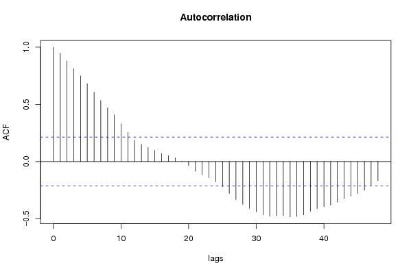
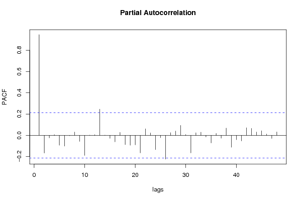
Title produced by software

(Partial) Autocorrelation Function

Date of computation

Wed, 10 Dec 2008 14:31:46 -0700

Cite this page as follows

Statistical Computations at FreeStatistics.org, Office for Research Development and Education, URL https://freestatistics.org/blog/index.php?v=date/2008/Dec/10/t1228944813fzarmg720suo4zn.htm/, Retrieved Fri, 17 May 2024 06:59:51 +0000

Statistical Computations at FreeStatistics.org, Office for Research Development and Education, URL https://freestatistics.org/blog/index.php?pk=32135, Retrieved Fri, 17 May 2024 06:59:51 +0000

QR Codes:

Paste this QR Code to cite your computation.

Original text written by user:

IsPrivate?

No (this computation is public)

User-defined keywords

Estimated Impact

195

Family? (F = Feedback message, R = changed R code, M = changed R Module, P = changed Parameters, D = changed Data)

-       [(Partial) Autocorrelation Function] [autocorelation - ...] [2008-12-10 21:31:46] [9e20205489828c19845a9d736cd20362] [Current]
-   PD    [(Partial) Autocorrelation Function] [verbetering opgav...] [2009-01-26 17:07:31] [65364f12da24daf6c8f7985fc762862c] 

Feedback Forum

Post a new message

Dataseries X:

Download CSV

Histogram

Boxplots

Summary of computational transaction
Raw Input	view raw input (R code)
Raw Output	view raw output of R engine
Computing time	7 seconds
R Server	'Sir Ronald Aylmer Fisher' @ 193.190.124.24

\begin{tabular}{lllllllll}
\hline
Summary of computational transaction \tabularnewline
Raw Input & view raw input (R code)  \tabularnewline
Raw Output & view raw output of R engine  \tabularnewline
Computing time & 7 seconds \tabularnewline
R Server & 'Sir Ronald Aylmer Fisher' @ 193.190.124.24 \tabularnewline
\hline
\end{tabular}
%Source: https://freestatistics.org/blog/index.php?pk=32135&T=0

[TABLE]
[ROW][C]Summary of computational transaction[/C][/ROW]
[ROW][C]Raw Input[/C][C]view raw input (R code) [/C][/ROW]
[ROW][C]Raw Output[/C][C]view raw output of R engine [/C][/ROW]
[ROW][C]Computing time[/C][C]7 seconds[/C][/ROW]
[ROW][C]R Server[/C][C]'Sir Ronald Aylmer Fisher' @ 193.190.124.24[/C][/ROW]
[/TABLE]
Source: https://freestatistics.org/blog/index.php?pk=32135&T=0

Globally Unique Identifier (entire table): ba.freestatistics.org/blog/index.php?pk=32135&T=0

As an alternative you can also use a QR Code:

The GUIDs for individual cells are displayed in the table below:

Summary of computational transaction
Raw Input	view raw input (R code)
Raw Output	view raw output of R engine
Computing time	7 seconds
R Server	'Sir Ronald Aylmer Fisher' @ 193.190.124.24

Autocorrelation Function
Time lag k	ACF(k)	T-STAT	P-value
1	0.947243	8.6816	0
2	0.880191	8.0671	0
3	0.812508	7.4468	0
4	0.749299	6.8674	0
5	0.681582	6.2468	0
6	0.606493	5.5586	0
7	0.533773	4.8921	2e-06
8	0.469999	4.3076	2.2e-05
9	0.407491	3.7347	0.000171
10	0.330117	3.0256	0.001646
11	0.253915	2.3272	0.011182
12	0.18551	1.7002	0.046394
13	0.150019	1.3749	0.086402
14	0.124113	1.1375	0.129279
15	0.098368	0.9016	0.184936
16	0.069994	0.6415	0.261471
17	0.050916	0.4667	0.320978
18	0.031669	0.2903	0.38617
19	0.003386	0.031	0.487658
20	-0.034868	-0.3196	0.375043
21	-0.084608	-0.7754	0.220126
22	-0.117386	-1.0759	0.142535
23	-0.141747	-1.2991	0.098727
24	-0.176254	-1.6154	0.054987
25	-0.220494	-2.0209	0.02324
26	-0.280202	-2.5681	0.005998
27	-0.333172	-3.0536	0.001514
28	-0.375359	-3.4402	0.000454
29	-0.409749	-3.7554	0.000159
30	-0.438782	-4.0215	6.3e-05
31	-0.465522	-4.2666	2.6e-05
32	-0.477426	-4.3757	1.7e-05
33	-0.475076	-4.3541	1.9e-05
34	-0.47525	-4.3557	1.9e-05
35	-0.484584	-4.4413	1.4e-05
36	-0.48131	-4.4113	1.5e-05
37	-0.466457	-4.2752	2.5e-05
38	-0.434145	-3.979	7.3e-05
39	-0.412291	-3.7787	0.000147
40	-0.395997	-3.6294	0.000244
41	-0.381896	-3.5001	0.000373
42	-0.354905	-3.2528	0.000823
43	-0.323593	-2.9658	0.001965
44	-0.30233	-2.7709	0.003441
45	-0.279725	-2.5637	0.006068
46	-0.251119	-2.3015	0.011918
47	-0.207903	-1.9055	0.030071
48	-0.167306	-1.5334	0.064469

\begin{tabular}{lllllllll}
\hline
Autocorrelation Function \tabularnewline
Time lag k & ACF(k) & T-STAT & P-value \tabularnewline
1 & 0.947243 & 8.6816 & 0 \tabularnewline
2 & 0.880191 & 8.0671 & 0 \tabularnewline
3 & 0.812508 & 7.4468 & 0 \tabularnewline
4 & 0.749299 & 6.8674 & 0 \tabularnewline
5 & 0.681582 & 6.2468 & 0 \tabularnewline
6 & 0.606493 & 5.5586 & 0 \tabularnewline
7 & 0.533773 & 4.8921 & 2e-06 \tabularnewline
8 & 0.469999 & 4.3076 & 2.2e-05 \tabularnewline
9 & 0.407491 & 3.7347 & 0.000171 \tabularnewline
10 & 0.330117 & 3.0256 & 0.001646 \tabularnewline
11 & 0.253915 & 2.3272 & 0.011182 \tabularnewline
12 & 0.18551 & 1.7002 & 0.046394 \tabularnewline
13 & 0.150019 & 1.3749 & 0.086402 \tabularnewline
14 & 0.124113 & 1.1375 & 0.129279 \tabularnewline
15 & 0.098368 & 0.9016 & 0.184936 \tabularnewline
16 & 0.069994 & 0.6415 & 0.261471 \tabularnewline
17 & 0.050916 & 0.4667 & 0.320978 \tabularnewline
18 & 0.031669 & 0.2903 & 0.38617 \tabularnewline
19 & 0.003386 & 0.031 & 0.487658 \tabularnewline
20 & -0.034868 & -0.3196 & 0.375043 \tabularnewline
21 & -0.084608 & -0.7754 & 0.220126 \tabularnewline
22 & -0.117386 & -1.0759 & 0.142535 \tabularnewline
23 & -0.141747 & -1.2991 & 0.098727 \tabularnewline
24 & -0.176254 & -1.6154 & 0.054987 \tabularnewline
25 & -0.220494 & -2.0209 & 0.02324 \tabularnewline
26 & -0.280202 & -2.5681 & 0.005998 \tabularnewline
27 & -0.333172 & -3.0536 & 0.001514 \tabularnewline
28 & -0.375359 & -3.4402 & 0.000454 \tabularnewline
29 & -0.409749 & -3.7554 & 0.000159 \tabularnewline
30 & -0.438782 & -4.0215 & 6.3e-05 \tabularnewline
31 & -0.465522 & -4.2666 & 2.6e-05 \tabularnewline
32 & -0.477426 & -4.3757 & 1.7e-05 \tabularnewline
33 & -0.475076 & -4.3541 & 1.9e-05 \tabularnewline
34 & -0.47525 & -4.3557 & 1.9e-05 \tabularnewline
35 & -0.484584 & -4.4413 & 1.4e-05 \tabularnewline
36 & -0.48131 & -4.4113 & 1.5e-05 \tabularnewline
37 & -0.466457 & -4.2752 & 2.5e-05 \tabularnewline
38 & -0.434145 & -3.979 & 7.3e-05 \tabularnewline
39 & -0.412291 & -3.7787 & 0.000147 \tabularnewline
40 & -0.395997 & -3.6294 & 0.000244 \tabularnewline
41 & -0.381896 & -3.5001 & 0.000373 \tabularnewline
42 & -0.354905 & -3.2528 & 0.000823 \tabularnewline
43 & -0.323593 & -2.9658 & 0.001965 \tabularnewline
44 & -0.30233 & -2.7709 & 0.003441 \tabularnewline
45 & -0.279725 & -2.5637 & 0.006068 \tabularnewline
46 & -0.251119 & -2.3015 & 0.011918 \tabularnewline
47 & -0.207903 & -1.9055 & 0.030071 \tabularnewline
48 & -0.167306 & -1.5334 & 0.064469 \tabularnewline
\hline
\end{tabular}
%Source: https://freestatistics.org/blog/index.php?pk=32135&T=1

[TABLE]
[ROW][C]Autocorrelation Function[/C][/ROW]
[ROW][C]Time lag k[/C][C]ACF(k)[/C][C]T-STAT[/C][C]P-value[/C][/ROW]
[ROW][C]1[/C][C]0.947243[/C][C]8.6816[/C][C]0[/C][/ROW]
[ROW][C]2[/C][C]0.880191[/C][C]8.0671[/C][C]0[/C][/ROW]
[ROW][C]3[/C][C]0.812508[/C][C]7.4468[/C][C]0[/C][/ROW]
[ROW][C]4[/C][C]0.749299[/C][C]6.8674[/C][C]0[/C][/ROW]
[ROW][C]5[/C][C]0.681582[/C][C]6.2468[/C][C]0[/C][/ROW]
[ROW][C]6[/C][C]0.606493[/C][C]5.5586[/C][C]0[/C][/ROW]
[ROW][C]7[/C][C]0.533773[/C][C]4.8921[/C][C]2e-06[/C][/ROW]
[ROW][C]8[/C][C]0.469999[/C][C]4.3076[/C][C]2.2e-05[/C][/ROW]
[ROW][C]9[/C][C]0.407491[/C][C]3.7347[/C][C]0.000171[/C][/ROW]
[ROW][C]10[/C][C]0.330117[/C][C]3.0256[/C][C]0.001646[/C][/ROW]
[ROW][C]11[/C][C]0.253915[/C][C]2.3272[/C][C]0.011182[/C][/ROW]
[ROW][C]12[/C][C]0.18551[/C][C]1.7002[/C][C]0.046394[/C][/ROW]
[ROW][C]13[/C][C]0.150019[/C][C]1.3749[/C][C]0.086402[/C][/ROW]
[ROW][C]14[/C][C]0.124113[/C][C]1.1375[/C][C]0.129279[/C][/ROW]
[ROW][C]15[/C][C]0.098368[/C][C]0.9016[/C][C]0.184936[/C][/ROW]
[ROW][C]16[/C][C]0.069994[/C][C]0.6415[/C][C]0.261471[/C][/ROW]
[ROW][C]17[/C][C]0.050916[/C][C]0.4667[/C][C]0.320978[/C][/ROW]
[ROW][C]18[/C][C]0.031669[/C][C]0.2903[/C][C]0.38617[/C][/ROW]
[ROW][C]19[/C][C]0.003386[/C][C]0.031[/C][C]0.487658[/C][/ROW]
[ROW][C]20[/C][C]-0.034868[/C][C]-0.3196[/C][C]0.375043[/C][/ROW]
[ROW][C]21[/C][C]-0.084608[/C][C]-0.7754[/C][C]0.220126[/C][/ROW]
[ROW][C]22[/C][C]-0.117386[/C][C]-1.0759[/C][C]0.142535[/C][/ROW]
[ROW][C]23[/C][C]-0.141747[/C][C]-1.2991[/C][C]0.098727[/C][/ROW]
[ROW][C]24[/C][C]-0.176254[/C][C]-1.6154[/C][C]0.054987[/C][/ROW]
[ROW][C]25[/C][C]-0.220494[/C][C]-2.0209[/C][C]0.02324[/C][/ROW]
[ROW][C]26[/C][C]-0.280202[/C][C]-2.5681[/C][C]0.005998[/C][/ROW]
[ROW][C]27[/C][C]-0.333172[/C][C]-3.0536[/C][C]0.001514[/C][/ROW]
[ROW][C]28[/C][C]-0.375359[/C][C]-3.4402[/C][C]0.000454[/C][/ROW]
[ROW][C]29[/C][C]-0.409749[/C][C]-3.7554[/C][C]0.000159[/C][/ROW]
[ROW][C]30[/C][C]-0.438782[/C][C]-4.0215[/C][C]6.3e-05[/C][/ROW]
[ROW][C]31[/C][C]-0.465522[/C][C]-4.2666[/C][C]2.6e-05[/C][/ROW]
[ROW][C]32[/C][C]-0.477426[/C][C]-4.3757[/C][C]1.7e-05[/C][/ROW]
[ROW][C]33[/C][C]-0.475076[/C][C]-4.3541[/C][C]1.9e-05[/C][/ROW]
[ROW][C]34[/C][C]-0.47525[/C][C]-4.3557[/C][C]1.9e-05[/C][/ROW]
[ROW][C]35[/C][C]-0.484584[/C][C]-4.4413[/C][C]1.4e-05[/C][/ROW]
[ROW][C]36[/C][C]-0.48131[/C][C]-4.4113[/C][C]1.5e-05[/C][/ROW]
[ROW][C]37[/C][C]-0.466457[/C][C]-4.2752[/C][C]2.5e-05[/C][/ROW]
[ROW][C]38[/C][C]-0.434145[/C][C]-3.979[/C][C]7.3e-05[/C][/ROW]
[ROW][C]39[/C][C]-0.412291[/C][C]-3.7787[/C][C]0.000147[/C][/ROW]
[ROW][C]40[/C][C]-0.395997[/C][C]-3.6294[/C][C]0.000244[/C][/ROW]
[ROW][C]41[/C][C]-0.381896[/C][C]-3.5001[/C][C]0.000373[/C][/ROW]
[ROW][C]42[/C][C]-0.354905[/C][C]-3.2528[/C][C]0.000823[/C][/ROW]
[ROW][C]43[/C][C]-0.323593[/C][C]-2.9658[/C][C]0.001965[/C][/ROW]
[ROW][C]44[/C][C]-0.30233[/C][C]-2.7709[/C][C]0.003441[/C][/ROW]
[ROW][C]45[/C][C]-0.279725[/C][C]-2.5637[/C][C]0.006068[/C][/ROW]
[ROW][C]46[/C][C]-0.251119[/C][C]-2.3015[/C][C]0.011918[/C][/ROW]
[ROW][C]47[/C][C]-0.207903[/C][C]-1.9055[/C][C]0.030071[/C][/ROW]
[ROW][C]48[/C][C]-0.167306[/C][C]-1.5334[/C][C]0.064469[/C][/ROW]
[/TABLE]
Source: https://freestatistics.org/blog/index.php?pk=32135&T=1

Globally Unique Identifier (entire table): ba.freestatistics.org/blog/index.php?pk=32135&T=1

As an alternative you can also use a QR Code:

The GUIDs for individual cells are displayed in the table below:

Autocorrelation Function
Time lag k	ACF(k)	T-STAT	P-value
1	0.947243	8.6816	0
2	0.880191	8.0671	0
3	0.812508	7.4468	0
4	0.749299	6.8674	0
5	0.681582	6.2468	0
6	0.606493	5.5586	0
7	0.533773	4.8921	2e-06
8	0.469999	4.3076	2.2e-05
9	0.407491	3.7347	0.000171
10	0.330117	3.0256	0.001646
11	0.253915	2.3272	0.011182
12	0.18551	1.7002	0.046394
13	0.150019	1.3749	0.086402
14	0.124113	1.1375	0.129279
15	0.098368	0.9016	0.184936
16	0.069994	0.6415	0.261471
17	0.050916	0.4667	0.320978
18	0.031669	0.2903	0.38617
19	0.003386	0.031	0.487658
20	-0.034868	-0.3196	0.375043
21	-0.084608	-0.7754	0.220126
22	-0.117386	-1.0759	0.142535
23	-0.141747	-1.2991	0.098727
24	-0.176254	-1.6154	0.054987
25	-0.220494	-2.0209	0.02324
26	-0.280202	-2.5681	0.005998
27	-0.333172	-3.0536	0.001514
28	-0.375359	-3.4402	0.000454
29	-0.409749	-3.7554	0.000159
30	-0.438782	-4.0215	6.3e-05
31	-0.465522	-4.2666	2.6e-05
32	-0.477426	-4.3757	1.7e-05
33	-0.475076	-4.3541	1.9e-05
34	-0.47525	-4.3557	1.9e-05
35	-0.484584	-4.4413	1.4e-05
36	-0.48131	-4.4113	1.5e-05
37	-0.466457	-4.2752	2.5e-05
38	-0.434145	-3.979	7.3e-05
39	-0.412291	-3.7787	0.000147
40	-0.395997	-3.6294	0.000244
41	-0.381896	-3.5001	0.000373
42	-0.354905	-3.2528	0.000823
43	-0.323593	-2.9658	0.001965
44	-0.30233	-2.7709	0.003441
45	-0.279725	-2.5637	0.006068
46	-0.251119	-2.3015	0.011918
47	-0.207903	-1.9055	0.030071
48	-0.167306	-1.5334	0.064469

Partial Autocorrelation Function
Time lag k	PACF(k)	T-STAT	P-value
1	0.947243	8.6816	0
2	-0.166249	-1.5237	0.06567
3	-0.023821	-0.2183	0.413854
4	0.006559	0.0601	0.476103
5	-0.092905	-0.8515	0.198459
6	-0.101482	-0.9301	0.177493
7	-0.003406	-0.0312	0.487586
8	0.030756	0.2819	0.389362
9	-0.057003	-0.5224	0.30137
10	-0.189114	-1.7333	0.043359
11	0.001393	0.0128	0.494921
12	0.006167	0.0565	0.477531
13	0.2463	2.2574	0.01329
14	0.001818	0.0167	0.493375
15	-0.027705	-0.2539	0.400088
16	-0.060934	-0.5585	0.289004
17	0.027315	0.2503	0.401466
18	-0.087339	-0.8005	0.212847
19	-0.093159	-0.8538	0.197818
20	-0.089318	-0.8186	0.207663
21	-0.165313	-1.5151	0.066748
22	0.061575	0.5643	0.287011
23	0.022592	0.2071	0.418234
24	-0.134152	-1.2295	0.111154
25	-0.022332	-0.2047	0.41916
26	-0.223632	-2.0496	0.021761
27	0.025566	0.2343	0.407654
28	0.040245	0.3689	0.356583
29	0.093618	0.858	0.19666
30	0.007701	0.0706	0.471948
31	-0.164948	-1.5118	0.067172
32	0.023879	0.2189	0.413647
33	0.029532	0.2707	0.393656
34	-0.015352	-0.1407	0.444221
35	-0.071254	-0.6531	0.257753
36	0.018064	0.1656	0.434449
37	-0.026795	-0.2456	0.403302
38	0.068348	0.6264	0.266369
39	-0.112012	-1.0266	0.153776
40	-0.040889	-0.3748	0.354394
41	-0.052645	-0.4825	0.315353
42	0.071268	0.6532	0.257712
43	0.065624	0.6015	0.274578
44	0.03116	0.2856	0.387948
45	0.043089	0.3949	0.346954
46	0.011998	0.11	0.456351
47	-0.029324	-0.2688	0.394387
48	0.032021	0.2935	0.384942

\begin{tabular}{lllllllll}
\hline
Partial Autocorrelation Function \tabularnewline
Time lag k & PACF(k) & T-STAT & P-value \tabularnewline
1 & 0.947243 & 8.6816 & 0 \tabularnewline
2 & -0.166249 & -1.5237 & 0.06567 \tabularnewline
3 & -0.023821 & -0.2183 & 0.413854 \tabularnewline
4 & 0.006559 & 0.0601 & 0.476103 \tabularnewline
5 & -0.092905 & -0.8515 & 0.198459 \tabularnewline
6 & -0.101482 & -0.9301 & 0.177493 \tabularnewline
7 & -0.003406 & -0.0312 & 0.487586 \tabularnewline
8 & 0.030756 & 0.2819 & 0.389362 \tabularnewline
9 & -0.057003 & -0.5224 & 0.30137 \tabularnewline
10 & -0.189114 & -1.7333 & 0.043359 \tabularnewline
11 & 0.001393 & 0.0128 & 0.494921 \tabularnewline
12 & 0.006167 & 0.0565 & 0.477531 \tabularnewline
13 & 0.2463 & 2.2574 & 0.01329 \tabularnewline
14 & 0.001818 & 0.0167 & 0.493375 \tabularnewline
15 & -0.027705 & -0.2539 & 0.400088 \tabularnewline
16 & -0.060934 & -0.5585 & 0.289004 \tabularnewline
17 & 0.027315 & 0.2503 & 0.401466 \tabularnewline
18 & -0.087339 & -0.8005 & 0.212847 \tabularnewline
19 & -0.093159 & -0.8538 & 0.197818 \tabularnewline
20 & -0.089318 & -0.8186 & 0.207663 \tabularnewline
21 & -0.165313 & -1.5151 & 0.066748 \tabularnewline
22 & 0.061575 & 0.5643 & 0.287011 \tabularnewline
23 & 0.022592 & 0.2071 & 0.418234 \tabularnewline
24 & -0.134152 & -1.2295 & 0.111154 \tabularnewline
25 & -0.022332 & -0.2047 & 0.41916 \tabularnewline
26 & -0.223632 & -2.0496 & 0.021761 \tabularnewline
27 & 0.025566 & 0.2343 & 0.407654 \tabularnewline
28 & 0.040245 & 0.3689 & 0.356583 \tabularnewline
29 & 0.093618 & 0.858 & 0.19666 \tabularnewline
30 & 0.007701 & 0.0706 & 0.471948 \tabularnewline
31 & -0.164948 & -1.5118 & 0.067172 \tabularnewline
32 & 0.023879 & 0.2189 & 0.413647 \tabularnewline
33 & 0.029532 & 0.2707 & 0.393656 \tabularnewline
34 & -0.015352 & -0.1407 & 0.444221 \tabularnewline
35 & -0.071254 & -0.6531 & 0.257753 \tabularnewline
36 & 0.018064 & 0.1656 & 0.434449 \tabularnewline
37 & -0.026795 & -0.2456 & 0.403302 \tabularnewline
38 & 0.068348 & 0.6264 & 0.266369 \tabularnewline
39 & -0.112012 & -1.0266 & 0.153776 \tabularnewline
40 & -0.040889 & -0.3748 & 0.354394 \tabularnewline
41 & -0.052645 & -0.4825 & 0.315353 \tabularnewline
42 & 0.071268 & 0.6532 & 0.257712 \tabularnewline
43 & 0.065624 & 0.6015 & 0.274578 \tabularnewline
44 & 0.03116 & 0.2856 & 0.387948 \tabularnewline
45 & 0.043089 & 0.3949 & 0.346954 \tabularnewline
46 & 0.011998 & 0.11 & 0.456351 \tabularnewline
47 & -0.029324 & -0.2688 & 0.394387 \tabularnewline
48 & 0.032021 & 0.2935 & 0.384942 \tabularnewline
\hline
\end{tabular}
%Source: https://freestatistics.org/blog/index.php?pk=32135&T=2

[TABLE]
[ROW][C]Partial Autocorrelation Function[/C][/ROW]
[ROW][C]Time lag k[/C][C]PACF(k)[/C][C]T-STAT[/C][C]P-value[/C][/ROW]
[ROW][C]1[/C][C]0.947243[/C][C]8.6816[/C][C]0[/C][/ROW]
[ROW][C]2[/C][C]-0.166249[/C][C]-1.5237[/C][C]0.06567[/C][/ROW]
[ROW][C]3[/C][C]-0.023821[/C][C]-0.2183[/C][C]0.413854[/C][/ROW]
[ROW][C]4[/C][C]0.006559[/C][C]0.0601[/C][C]0.476103[/C][/ROW]
[ROW][C]5[/C][C]-0.092905[/C][C]-0.8515[/C][C]0.198459[/C][/ROW]
[ROW][C]6[/C][C]-0.101482[/C][C]-0.9301[/C][C]0.177493[/C][/ROW]
[ROW][C]7[/C][C]-0.003406[/C][C]-0.0312[/C][C]0.487586[/C][/ROW]
[ROW][C]8[/C][C]0.030756[/C][C]0.2819[/C][C]0.389362[/C][/ROW]
[ROW][C]9[/C][C]-0.057003[/C][C]-0.5224[/C][C]0.30137[/C][/ROW]
[ROW][C]10[/C][C]-0.189114[/C][C]-1.7333[/C][C]0.043359[/C][/ROW]
[ROW][C]11[/C][C]0.001393[/C][C]0.0128[/C][C]0.494921[/C][/ROW]
[ROW][C]12[/C][C]0.006167[/C][C]0.0565[/C][C]0.477531[/C][/ROW]
[ROW][C]13[/C][C]0.2463[/C][C]2.2574[/C][C]0.01329[/C][/ROW]
[ROW][C]14[/C][C]0.001818[/C][C]0.0167[/C][C]0.493375[/C][/ROW]
[ROW][C]15[/C][C]-0.027705[/C][C]-0.2539[/C][C]0.400088[/C][/ROW]
[ROW][C]16[/C][C]-0.060934[/C][C]-0.5585[/C][C]0.289004[/C][/ROW]
[ROW][C]17[/C][C]0.027315[/C][C]0.2503[/C][C]0.401466[/C][/ROW]
[ROW][C]18[/C][C]-0.087339[/C][C]-0.8005[/C][C]0.212847[/C][/ROW]
[ROW][C]19[/C][C]-0.093159[/C][C]-0.8538[/C][C]0.197818[/C][/ROW]
[ROW][C]20[/C][C]-0.089318[/C][C]-0.8186[/C][C]0.207663[/C][/ROW]
[ROW][C]21[/C][C]-0.165313[/C][C]-1.5151[/C][C]0.066748[/C][/ROW]
[ROW][C]22[/C][C]0.061575[/C][C]0.5643[/C][C]0.287011[/C][/ROW]
[ROW][C]23[/C][C]0.022592[/C][C]0.2071[/C][C]0.418234[/C][/ROW]
[ROW][C]24[/C][C]-0.134152[/C][C]-1.2295[/C][C]0.111154[/C][/ROW]
[ROW][C]25[/C][C]-0.022332[/C][C]-0.2047[/C][C]0.41916[/C][/ROW]
[ROW][C]26[/C][C]-0.223632[/C][C]-2.0496[/C][C]0.021761[/C][/ROW]
[ROW][C]27[/C][C]0.025566[/C][C]0.2343[/C][C]0.407654[/C][/ROW]
[ROW][C]28[/C][C]0.040245[/C][C]0.3689[/C][C]0.356583[/C][/ROW]
[ROW][C]29[/C][C]0.093618[/C][C]0.858[/C][C]0.19666[/C][/ROW]
[ROW][C]30[/C][C]0.007701[/C][C]0.0706[/C][C]0.471948[/C][/ROW]
[ROW][C]31[/C][C]-0.164948[/C][C]-1.5118[/C][C]0.067172[/C][/ROW]
[ROW][C]32[/C][C]0.023879[/C][C]0.2189[/C][C]0.413647[/C][/ROW]
[ROW][C]33[/C][C]0.029532[/C][C]0.2707[/C][C]0.393656[/C][/ROW]
[ROW][C]34[/C][C]-0.015352[/C][C]-0.1407[/C][C]0.444221[/C][/ROW]
[ROW][C]35[/C][C]-0.071254[/C][C]-0.6531[/C][C]0.257753[/C][/ROW]
[ROW][C]36[/C][C]0.018064[/C][C]0.1656[/C][C]0.434449[/C][/ROW]
[ROW][C]37[/C][C]-0.026795[/C][C]-0.2456[/C][C]0.403302[/C][/ROW]
[ROW][C]38[/C][C]0.068348[/C][C]0.6264[/C][C]0.266369[/C][/ROW]
[ROW][C]39[/C][C]-0.112012[/C][C]-1.0266[/C][C]0.153776[/C][/ROW]
[ROW][C]40[/C][C]-0.040889[/C][C]-0.3748[/C][C]0.354394[/C][/ROW]
[ROW][C]41[/C][C]-0.052645[/C][C]-0.4825[/C][C]0.315353[/C][/ROW]
[ROW][C]42[/C][C]0.071268[/C][C]0.6532[/C][C]0.257712[/C][/ROW]
[ROW][C]43[/C][C]0.065624[/C][C]0.6015[/C][C]0.274578[/C][/ROW]
[ROW][C]44[/C][C]0.03116[/C][C]0.2856[/C][C]0.387948[/C][/ROW]
[ROW][C]45[/C][C]0.043089[/C][C]0.3949[/C][C]0.346954[/C][/ROW]
[ROW][C]46[/C][C]0.011998[/C][C]0.11[/C][C]0.456351[/C][/ROW]
[ROW][C]47[/C][C]-0.029324[/C][C]-0.2688[/C][C]0.394387[/C][/ROW]
[ROW][C]48[/C][C]0.032021[/C][C]0.2935[/C][C]0.384942[/C][/ROW]
[/TABLE]
Source: https://freestatistics.org/blog/index.php?pk=32135&T=2

Globally Unique Identifier (entire table): ba.freestatistics.org/blog/index.php?pk=32135&T=2

As an alternative you can also use a QR Code:

The GUIDs for individual cells are displayed in the table below:

Partial Autocorrelation Function
Time lag k	PACF(k)	T-STAT	P-value
1	0.947243	8.6816	0
2	-0.166249	-1.5237	0.06567
3	-0.023821	-0.2183	0.413854
4	0.006559	0.0601	0.476103
5	-0.092905	-0.8515	0.198459
6	-0.101482	-0.9301	0.177493
7	-0.003406	-0.0312	0.487586
8	0.030756	0.2819	0.389362
9	-0.057003	-0.5224	0.30137
10	-0.189114	-1.7333	0.043359
11	0.001393	0.0128	0.494921
12	0.006167	0.0565	0.477531
13	0.2463	2.2574	0.01329
14	0.001818	0.0167	0.493375
15	-0.027705	-0.2539	0.400088
16	-0.060934	-0.5585	0.289004
17	0.027315	0.2503	0.401466
18	-0.087339	-0.8005	0.212847
19	-0.093159	-0.8538	0.197818
20	-0.089318	-0.8186	0.207663
21	-0.165313	-1.5151	0.066748
22	0.061575	0.5643	0.287011
23	0.022592	0.2071	0.418234
24	-0.134152	-1.2295	0.111154
25	-0.022332	-0.2047	0.41916
26	-0.223632	-2.0496	0.021761
27	0.025566	0.2343	0.407654
28	0.040245	0.3689	0.356583
29	0.093618	0.858	0.19666
30	0.007701	0.0706	0.471948
31	-0.164948	-1.5118	0.067172
32	0.023879	0.2189	0.413647
33	0.029532	0.2707	0.393656
34	-0.015352	-0.1407	0.444221
35	-0.071254	-0.6531	0.257753
36	0.018064	0.1656	0.434449
37	-0.026795	-0.2456	0.403302
38	0.068348	0.6264	0.266369
39	-0.112012	-1.0266	0.153776
40	-0.040889	-0.3748	0.354394
41	-0.052645	-0.4825	0.315353
42	0.071268	0.6532	0.257712
43	0.065624	0.6015	0.274578
44	0.03116	0.2856	0.387948
45	0.043089	0.3949	0.346954
46	0.011998	0.11	0.456351
47	-0.029324	-0.2688	0.394387
48	0.032021	0.2935	0.384942

Figure 1

PNG link

Postscript link

PDF link

Figure 2

PNG link

Postscript link

PDF link

Parameters (Session):

par1 = 48 ; par2 = 1 ; par3 = 0 ; par4 = 1 ; par5 = 12 ;

Parameters (R input):

par1 = 48 ; par2 = 1 ; par3 = 0 ; par4 = 1 ; par5 = 12 ;

R code (references can be found in the software module):

if (par1 == 'Default') {
par1 = 10*log10(length(x))
} else {
par1 <- as.numeric(par1)
}
par2 <- as.numeric(par2)
par3 <- as.numeric(par3)
par4 <- as.numeric(par4)
par5 <- as.numeric(par5)
if (par2 == 0) {
x <- log(x)
} else {
x <- (x ^ par2 - 1) / par2
}
if (par3 > 0) x <- diff(x,lag=1,difference=par3)
if (par4 > 0) x <- diff(x,lag=par5,difference=par4)
bitmap(file='pic1.png')
racf <- acf(x,par1,main='Autocorrelation',xlab='lags',ylab='ACF')
dev.off()
bitmap(file='pic2.png')
rpacf <- pacf(x,par1,main='Partial Autocorrelation',xlab='lags',ylab='PACF')
dev.off()
(myacf <- c(racf$acf))
(mypacf <- c(rpacf$acf))
lengthx <- length(x)
sqrtn <- sqrt(lengthx)
load(file='createtable')
a<-table.start()
a<-table.row.start(a)
a<-table.element(a,'Autocorrelation Function',4,TRUE)
a<-table.row.end(a)
a<-table.row.start(a)
a<-table.element(a,'Time lag k',header=TRUE)
a<-table.element(a,hyperlink('basics.htm','ACF(k)','click here for more information about the Autocorrelation Function'),header=TRUE)
a<-table.element(a,'T-STAT',header=TRUE)
a<-table.element(a,'P-value',header=TRUE)
a<-table.row.end(a)
for (i in 2:(par1+1)) {
a<-table.row.start(a)
a<-table.element(a,i-1,header=TRUE)
a<-table.element(a,round(myacf[i],6))
mytstat <- myacf[i]*sqrtn
a<-table.element(a,round(mytstat,4))
a<-table.element(a,round(1-pt(abs(mytstat),lengthx),6))
a<-table.row.end(a)
}
a<-table.end(a)
table.save(a,file='mytable.tab')
a<-table.start()
a<-table.row.start(a)
a<-table.element(a,'Partial Autocorrelation Function',4,TRUE)
a<-table.row.end(a)
a<-table.row.start(a)
a<-table.element(a,'Time lag k',header=TRUE)
a<-table.element(a,hyperlink('basics.htm','PACF(k)','click here for more information about the Partial Autocorrelation Function'),header=TRUE)
a<-table.element(a,'T-STAT',header=TRUE)
a<-table.element(a,'P-value',header=TRUE)
a<-table.row.end(a)
for (i in 1:par1) {
a<-table.row.start(a)
a<-table.element(a,i,header=TRUE)
a<-table.element(a,round(mypacf[i],6))
mytstat <- mypacf[i]*sqrtn
a<-table.element(a,round(mytstat,4))
a<-table.element(a,round(1-pt(abs(mytstat),lengthx),6))
a<-table.row.end(a)
}
a<-table.end(a)
table.save(a,file='mytable1.tab')

Free Statistics

Description of Statistical Computation

Tree of Dependent Computations

Dataset

Tables (Output of Computation)

Figures (Output of Computation)

Input Parameters & R Code