Free Statistics
of Irreproducible Research!
Description of Statistical Computation | |||||||||||||||||||||||||||||||||||||||||||||
|---|---|---|---|---|---|---|---|---|---|---|---|---|---|---|---|---|---|---|---|---|---|---|---|---|---|---|---|---|---|---|---|---|---|---|---|---|---|---|---|---|---|---|---|---|---|
| Author's title | Box-Cox Linearity Plot: Duurzame consumptiegoederen vs niet-duurzame consum... | ||||||||||||||||||||||||||||||||||||||||||||
| Author | *The author of this computation has been verified* | ||||||||||||||||||||||||||||||||||||||||||||
| R Software Module | rwasp_boxcoxlin.wasp | ||||||||||||||||||||||||||||||||||||||||||||
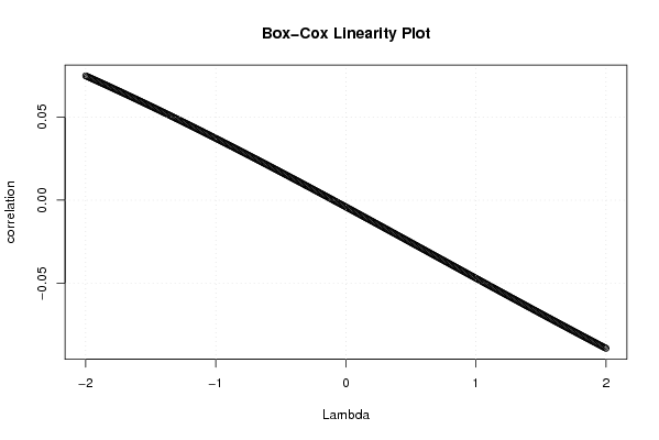
| Title produced by software | Box-Cox Linearity Plot | ||||||||||||||||||||||||||||||||||||||||||||
| Date of computation | Wed, 10 Dec 2008 08:39:29 -0700 | ||||||||||||||||||||||||||||||||||||||||||||
| Cite this page as follows | Statistical Computations at FreeStatistics.org, Office for Research Development and Education, URL https://freestatistics.org/blog/index.php?v=date/2008/Dec/10/t12289237518p0zmcosj4taa4r.htm/, Retrieved Fri, 17 May 2024 02:01:39 +0000 | ||||||||||||||||||||||||||||||||||||||||||||
| Statistical Computations at FreeStatistics.org, Office for Research Development and Education, URL https://freestatistics.org/blog/index.php?pk=32005, Retrieved Fri, 17 May 2024 02:01:39 +0000 | |||||||||||||||||||||||||||||||||||||||||||||
| QR Codes: | |||||||||||||||||||||||||||||||||||||||||||||
|
| |||||||||||||||||||||||||||||||||||||||||||||
| Original text written by user: | |||||||||||||||||||||||||||||||||||||||||||||
| IsPrivate? | No (this computation is public) | ||||||||||||||||||||||||||||||||||||||||||||
| User-defined keywords | |||||||||||||||||||||||||||||||||||||||||||||
| Estimated Impact | 160 | ||||||||||||||||||||||||||||||||||||||||||||
Tree of Dependent Computations | |||||||||||||||||||||||||||||||||||||||||||||
| Family? (F = Feedback message, R = changed R code, M = changed R Module, P = changed Parameters, D = changed Data) | |||||||||||||||||||||||||||||||||||||||||||||
| - [Box-Cox Linearity Plot] [Box-Cox Linearity...] [2008-12-10 15:39:29] [6aa66640011d9b98524a5838bcf7301d] [Current] | |||||||||||||||||||||||||||||||||||||||||||||
| Feedback Forum | |||||||||||||||||||||||||||||||||||||||||||||
Post a new message | |||||||||||||||||||||||||||||||||||||||||||||
Dataset | |||||||||||||||||||||||||||||||||||||||||||||
| Dataseries X: | |||||||||||||||||||||||||||||||||||||||||||||
85,0 95,9 108,9 96,2 100,1 105,7 64,5 66,8 110,3 96,1 102,5 97,6 83,6 86,5 96,0 91,1 87,2 84,5 59,2 61,5 98,8 97,9 92,7 84,2 74,5 79,7 86,8 79,8 87,0 91,4 58,7 62,8 87,9 90,4 80,6 73,5 71,4 70,6 78,3 76,0 77,4 80,9 63,4 58,1 88,2 81,2 84,9 76,4 71,5 76,1 82,9 78,0 82,0 84,7 55,7 59,5 83,2 87,6 76,2 76,4 68,3 70,0 76,3 70,9 72,4 80,1 57,4 62,7 82,6 88,9 80,4 72,0 69,4 69,2 77,3 79,4 78,6 76,1 61,8 59,4 78,1 | |||||||||||||||||||||||||||||||||||||||||||||
| Dataseries Y: | |||||||||||||||||||||||||||||||||||||||||||||
99,5 98,2 108,9 100,0 105,0 108,4 96,7 100,5 115,6 114,9 110,7 107,7 113,5 106,9 119,6 109,4 106,9 118,7 108,9 113,1 125,1 126,5 122,7 127,5 107,1 112,0 122,1 111,5 113,2 128,2 115,1 117,4 132,0 130,8 128,0 132,7 117,0 110,9 123,5 117,4 122,7 123,5 111,5 113,8 131,2 127,0 126,2 121,2 118,8 117,9 135,2 120,7 126,4 129,6 113,4 120,5 135,5 137,6 130,6 133,1 121,5 120,5 136,9 123,7 128,5 135,0 120,9 121,1 132,2 134,5 133,6 136,1 124,5 124,6 133,5 132,3 125,3 135,5 121,2 117,5 135,9 | |||||||||||||||||||||||||||||||||||||||||||||
Tables (Output of Computation) | |||||||||||||||||||||||||||||||||||||||||||||
| |||||||||||||||||||||||||||||||||||||||||||||
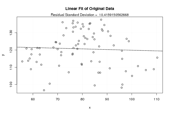
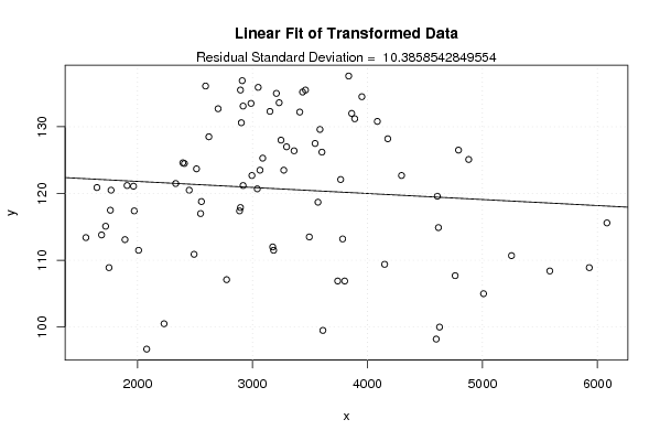
Figures (Output of Computation) | |||||||||||||||||||||||||||||||||||||||||||||
Input Parameters & R Code | |||||||||||||||||||||||||||||||||||||||||||||
| Parameters (Session): | |||||||||||||||||||||||||||||||||||||||||||||
| Parameters (R input): | |||||||||||||||||||||||||||||||||||||||||||||
| R code (references can be found in the software module): | |||||||||||||||||||||||||||||||||||||||||||||
n <- length(x) | |||||||||||||||||||||||||||||||||||||||||||||