Repository of Reproducible Computations

Free Statistics

of Irreproducible Research!

Author's title

Author

*The author of this computation has been verified*

R Software Module

rwasp_autocorrelation.wasp

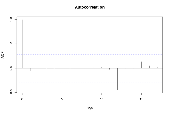
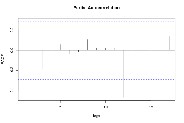
Title produced by software

(Partial) Autocorrelation Function

Date of computation

Mon, 08 Dec 2008 14:39:21 -0700

Cite this page as follows

Statistical Computations at FreeStatistics.org, Office for Research Development and Education, URL https://freestatistics.org/blog/index.php?v=date/2008/Dec/08/t1228772436enmlcunbt431hhq.htm/, Retrieved Thu, 16 May 2024 11:30:47 +0000

Statistical Computations at FreeStatistics.org, Office for Research Development and Education, URL https://freestatistics.org/blog/index.php?pk=31079, Retrieved Thu, 16 May 2024 11:30:47 +0000

QR Codes:

Paste this QR Code to cite your computation.

Original text written by user:

IsPrivate?

No (this computation is public)

User-defined keywords

Estimated Impact

166

Family? (F = Feedback message, R = changed R code, M = changed R Module, P = changed Parameters, D = changed Data)

-     [Univariate Data Series] [data set] [2008-12-01 19:54:57] [b98453cac15ba1066b407e146608df68]
F RMP   [Standard Deviation-Mean Plot] [SMP Analysis] [2008-12-08 10:07:54] [23bfa928dab4b48567707937094f7011]
F RMPD      [(Partial) Autocorrelation Function] [ACF] [2008-12-08 21:39:21] [63302faa1e3976bf98d1de42298c0b24] [Current]

Feedback Forum

2008-12-14 23:41:02 [df2ed12c9b09685cd516719b004050c5] [reply] 
hier heb je dezelfde fout gemaakt als bij de werkloosheidsdata.

Post a new message

Dataseries X:

Download CSV

Histogram

Boxplots

Summary of computational transaction
Raw Input	view raw input (R code)
Raw Output	view raw output of R engine
Computing time	1 seconds
R Server	'George Udny Yule' @ 72.249.76.132

\begin{tabular}{lllllllll}
\hline
Summary of computational transaction \tabularnewline
Raw Input & view raw input (R code)  \tabularnewline
Raw Output & view raw output of R engine  \tabularnewline
Computing time & 1 seconds \tabularnewline
R Server & 'George Udny Yule' @ 72.249.76.132 \tabularnewline
\hline
\end{tabular}
%Source: https://freestatistics.org/blog/index.php?pk=31079&T=0

[TABLE]
[ROW][C]Summary of computational transaction[/C][/ROW]
[ROW][C]Raw Input[/C][C]view raw input (R code) [/C][/ROW]
[ROW][C]Raw Output[/C][C]view raw output of R engine [/C][/ROW]
[ROW][C]Computing time[/C][C]1 seconds[/C][/ROW]
[ROW][C]R Server[/C][C]'George Udny Yule' @ 72.249.76.132[/C][/ROW]
[/TABLE]
Source: https://freestatistics.org/blog/index.php?pk=31079&T=0

Globally Unique Identifier (entire table): ba.freestatistics.org/blog/index.php?pk=31079&T=0

As an alternative you can also use a QR Code:

The GUIDs for individual cells are displayed in the table below:

Summary of computational transaction
Raw Input	view raw input (R code)
Raw Output	view raw output of R engine
Computing time	1 seconds
R Server	'George Udny Yule' @ 72.249.76.132

Autocorrelation Function
Time lag k	ACF(k)	T-STAT	P-value
1	-0.05527	-0.3789	0.353231
2	0.004993	0.0342	0.486419
3	-0.181941	-1.2473	0.109229
4	-0.043913	-0.3011	0.382351
5	0.061704	0.423	0.337105
6	-0.005245	-0.036	0.485733
7	0.009765	0.0669	0.473454
8	0.08191	0.5615	0.288547
9	0.012737	0.0873	0.465395
10	0.026818	0.1839	0.427458
11	-0.023499	-0.1611	0.436351
12	-0.452428	-3.1017	0.001625
13	0.001411	0.0097	0.496162
14	0.005406	0.0371	0.485295
15	0.136044	0.9327	0.177879
16	0.050817	0.3484	0.364554
17	0.02714	0.1861	0.426597

\begin{tabular}{lllllllll}
\hline
Autocorrelation Function \tabularnewline
Time lag k & ACF(k) & T-STAT & P-value \tabularnewline
1 & -0.05527 & -0.3789 & 0.353231 \tabularnewline
2 & 0.004993 & 0.0342 & 0.486419 \tabularnewline
3 & -0.181941 & -1.2473 & 0.109229 \tabularnewline
4 & -0.043913 & -0.3011 & 0.382351 \tabularnewline
5 & 0.061704 & 0.423 & 0.337105 \tabularnewline
6 & -0.005245 & -0.036 & 0.485733 \tabularnewline
7 & 0.009765 & 0.0669 & 0.473454 \tabularnewline
8 & 0.08191 & 0.5615 & 0.288547 \tabularnewline
9 & 0.012737 & 0.0873 & 0.465395 \tabularnewline
10 & 0.026818 & 0.1839 & 0.427458 \tabularnewline
11 & -0.023499 & -0.1611 & 0.436351 \tabularnewline
12 & -0.452428 & -3.1017 & 0.001625 \tabularnewline
13 & 0.001411 & 0.0097 & 0.496162 \tabularnewline
14 & 0.005406 & 0.0371 & 0.485295 \tabularnewline
15 & 0.136044 & 0.9327 & 0.177879 \tabularnewline
16 & 0.050817 & 0.3484 & 0.364554 \tabularnewline
17 & 0.02714 & 0.1861 & 0.426597 \tabularnewline
\hline
\end{tabular}
%Source: https://freestatistics.org/blog/index.php?pk=31079&T=1

[TABLE]
[ROW][C]Autocorrelation Function[/C][/ROW]
[ROW][C]Time lag k[/C][C]ACF(k)[/C][C]T-STAT[/C][C]P-value[/C][/ROW]
[ROW][C]1[/C][C]-0.05527[/C][C]-0.3789[/C][C]0.353231[/C][/ROW]
[ROW][C]2[/C][C]0.004993[/C][C]0.0342[/C][C]0.486419[/C][/ROW]
[ROW][C]3[/C][C]-0.181941[/C][C]-1.2473[/C][C]0.109229[/C][/ROW]
[ROW][C]4[/C][C]-0.043913[/C][C]-0.3011[/C][C]0.382351[/C][/ROW]
[ROW][C]5[/C][C]0.061704[/C][C]0.423[/C][C]0.337105[/C][/ROW]
[ROW][C]6[/C][C]-0.005245[/C][C]-0.036[/C][C]0.485733[/C][/ROW]
[ROW][C]7[/C][C]0.009765[/C][C]0.0669[/C][C]0.473454[/C][/ROW]
[ROW][C]8[/C][C]0.08191[/C][C]0.5615[/C][C]0.288547[/C][/ROW]
[ROW][C]9[/C][C]0.012737[/C][C]0.0873[/C][C]0.465395[/C][/ROW]
[ROW][C]10[/C][C]0.026818[/C][C]0.1839[/C][C]0.427458[/C][/ROW]
[ROW][C]11[/C][C]-0.023499[/C][C]-0.1611[/C][C]0.436351[/C][/ROW]
[ROW][C]12[/C][C]-0.452428[/C][C]-3.1017[/C][C]0.001625[/C][/ROW]
[ROW][C]13[/C][C]0.001411[/C][C]0.0097[/C][C]0.496162[/C][/ROW]
[ROW][C]14[/C][C]0.005406[/C][C]0.0371[/C][C]0.485295[/C][/ROW]
[ROW][C]15[/C][C]0.136044[/C][C]0.9327[/C][C]0.177879[/C][/ROW]
[ROW][C]16[/C][C]0.050817[/C][C]0.3484[/C][C]0.364554[/C][/ROW]
[ROW][C]17[/C][C]0.02714[/C][C]0.1861[/C][C]0.426597[/C][/ROW]
[/TABLE]
Source: https://freestatistics.org/blog/index.php?pk=31079&T=1

Globally Unique Identifier (entire table): ba.freestatistics.org/blog/index.php?pk=31079&T=1

As an alternative you can also use a QR Code:

The GUIDs for individual cells are displayed in the table below:

Autocorrelation Function
Time lag k	ACF(k)	T-STAT	P-value
1	-0.05527	-0.3789	0.353231
2	0.004993	0.0342	0.486419
3	-0.181941	-1.2473	0.109229
4	-0.043913	-0.3011	0.382351
5	0.061704	0.423	0.337105
6	-0.005245	-0.036	0.485733
7	0.009765	0.0669	0.473454
8	0.08191	0.5615	0.288547
9	0.012737	0.0873	0.465395
10	0.026818	0.1839	0.427458
11	-0.023499	-0.1611	0.436351
12	-0.452428	-3.1017	0.001625
13	0.001411	0.0097	0.496162
14	0.005406	0.0371	0.485295
15	0.136044	0.9327	0.177879
16	0.050817	0.3484	0.364554
17	0.02714	0.1861	0.426597

Partial Autocorrelation Function
Time lag k	PACF(k)	T-STAT	P-value
1	-0.05527	-0.3789	0.353231
2	0.001944	0.0133	0.49471
3	-0.182115	-1.2485	0.109012
4	-0.066305	-0.4546	0.325757
5	0.056748	0.389	0.349499
6	-0.032957	-0.2259	0.411114
7	-0.012984	-0.089	0.464725
8	0.105635	0.7242	0.236266
9	0.02455	0.1683	0.433531
10	0.023855	0.1635	0.435398
11	0.018609	0.1276	0.449515
12	-0.463206	-3.1756	0.00132
13	-0.071074	-0.4873	0.314171
14	0.014379	0.0986	0.460947
15	-0.051365	-0.3521	0.363153
16	0.023129	0.1586	0.437346
17	0.136275	0.9343	0.177474

\begin{tabular}{lllllllll}
\hline
Partial Autocorrelation Function \tabularnewline
Time lag k & PACF(k) & T-STAT & P-value \tabularnewline
1 & -0.05527 & -0.3789 & 0.353231 \tabularnewline
2 & 0.001944 & 0.0133 & 0.49471 \tabularnewline
3 & -0.182115 & -1.2485 & 0.109012 \tabularnewline
4 & -0.066305 & -0.4546 & 0.325757 \tabularnewline
5 & 0.056748 & 0.389 & 0.349499 \tabularnewline
6 & -0.032957 & -0.2259 & 0.411114 \tabularnewline
7 & -0.012984 & -0.089 & 0.464725 \tabularnewline
8 & 0.105635 & 0.7242 & 0.236266 \tabularnewline
9 & 0.02455 & 0.1683 & 0.433531 \tabularnewline
10 & 0.023855 & 0.1635 & 0.435398 \tabularnewline
11 & 0.018609 & 0.1276 & 0.449515 \tabularnewline
12 & -0.463206 & -3.1756 & 0.00132 \tabularnewline
13 & -0.071074 & -0.4873 & 0.314171 \tabularnewline
14 & 0.014379 & 0.0986 & 0.460947 \tabularnewline
15 & -0.051365 & -0.3521 & 0.363153 \tabularnewline
16 & 0.023129 & 0.1586 & 0.437346 \tabularnewline
17 & 0.136275 & 0.9343 & 0.177474 \tabularnewline
\hline
\end{tabular}
%Source: https://freestatistics.org/blog/index.php?pk=31079&T=2

[TABLE]
[ROW][C]Partial Autocorrelation Function[/C][/ROW]
[ROW][C]Time lag k[/C][C]PACF(k)[/C][C]T-STAT[/C][C]P-value[/C][/ROW]
[ROW][C]1[/C][C]-0.05527[/C][C]-0.3789[/C][C]0.353231[/C][/ROW]
[ROW][C]2[/C][C]0.001944[/C][C]0.0133[/C][C]0.49471[/C][/ROW]
[ROW][C]3[/C][C]-0.182115[/C][C]-1.2485[/C][C]0.109012[/C][/ROW]
[ROW][C]4[/C][C]-0.066305[/C][C]-0.4546[/C][C]0.325757[/C][/ROW]
[ROW][C]5[/C][C]0.056748[/C][C]0.389[/C][C]0.349499[/C][/ROW]
[ROW][C]6[/C][C]-0.032957[/C][C]-0.2259[/C][C]0.411114[/C][/ROW]
[ROW][C]7[/C][C]-0.012984[/C][C]-0.089[/C][C]0.464725[/C][/ROW]
[ROW][C]8[/C][C]0.105635[/C][C]0.7242[/C][C]0.236266[/C][/ROW]
[ROW][C]9[/C][C]0.02455[/C][C]0.1683[/C][C]0.433531[/C][/ROW]
[ROW][C]10[/C][C]0.023855[/C][C]0.1635[/C][C]0.435398[/C][/ROW]
[ROW][C]11[/C][C]0.018609[/C][C]0.1276[/C][C]0.449515[/C][/ROW]
[ROW][C]12[/C][C]-0.463206[/C][C]-3.1756[/C][C]0.00132[/C][/ROW]
[ROW][C]13[/C][C]-0.071074[/C][C]-0.4873[/C][C]0.314171[/C][/ROW]
[ROW][C]14[/C][C]0.014379[/C][C]0.0986[/C][C]0.460947[/C][/ROW]
[ROW][C]15[/C][C]-0.051365[/C][C]-0.3521[/C][C]0.363153[/C][/ROW]
[ROW][C]16[/C][C]0.023129[/C][C]0.1586[/C][C]0.437346[/C][/ROW]
[ROW][C]17[/C][C]0.136275[/C][C]0.9343[/C][C]0.177474[/C][/ROW]
[/TABLE]
Source: https://freestatistics.org/blog/index.php?pk=31079&T=2

Globally Unique Identifier (entire table): ba.freestatistics.org/blog/index.php?pk=31079&T=2

As an alternative you can also use a QR Code:

The GUIDs for individual cells are displayed in the table below:

Partial Autocorrelation Function
Time lag k	PACF(k)	T-STAT	P-value
1	-0.05527	-0.3789	0.353231
2	0.001944	0.0133	0.49471
3	-0.182115	-1.2485	0.109012
4	-0.066305	-0.4546	0.325757
5	0.056748	0.389	0.349499
6	-0.032957	-0.2259	0.411114
7	-0.012984	-0.089	0.464725
8	0.105635	0.7242	0.236266
9	0.02455	0.1683	0.433531
10	0.023855	0.1635	0.435398
11	0.018609	0.1276	0.449515
12	-0.463206	-3.1756	0.00132
13	-0.071074	-0.4873	0.314171
14	0.014379	0.0986	0.460947
15	-0.051365	-0.3521	0.363153
16	0.023129	0.1586	0.437346
17	0.136275	0.9343	0.177474

Figure 1

PNG link

Postscript link

PDF link

Figure 2

PNG link

Postscript link

PDF link

Parameters (Session):

par1 = Default ; par2 = 1 ; par3 = 1 ; par4 = 1 ; par5 = 12 ;

Parameters (R input):

par1 = Default ; par2 = 1 ; par3 = 1 ; par4 = 1 ; par5 = 12 ;

R code (references can be found in the software module):

if (par1 == 'Default') {
par1 = 10*log10(length(x))
} else {
par1 <- as.numeric(par1)
}
par2 <- as.numeric(par2)
par3 <- as.numeric(par3)
par4 <- as.numeric(par4)
par5 <- as.numeric(par5)
if (par2 == 0) {
x <- log(x)
} else {
x <- (x ^ par2 - 1) / par2
}
if (par3 > 0) x <- diff(x,lag=1,difference=par3)
if (par4 > 0) x <- diff(x,lag=par5,difference=par4)
bitmap(file='pic1.png')
racf <- acf(x,par1,main='Autocorrelation',xlab='lags',ylab='ACF')
dev.off()
bitmap(file='pic2.png')
rpacf <- pacf(x,par1,main='Partial Autocorrelation',xlab='lags',ylab='PACF')
dev.off()
(myacf <- c(racf$acf))
(mypacf <- c(rpacf$acf))
lengthx <- length(x)
sqrtn <- sqrt(lengthx)
load(file='createtable')
a<-table.start()
a<-table.row.start(a)
a<-table.element(a,'Autocorrelation Function',4,TRUE)
a<-table.row.end(a)
a<-table.row.start(a)
a<-table.element(a,'Time lag k',header=TRUE)
a<-table.element(a,hyperlink('basics.htm','ACF(k)','click here for more information about the Autocorrelation Function'),header=TRUE)
a<-table.element(a,'T-STAT',header=TRUE)
a<-table.element(a,'P-value',header=TRUE)
a<-table.row.end(a)
for (i in 2:(par1+1)) {
a<-table.row.start(a)
a<-table.element(a,i-1,header=TRUE)
a<-table.element(a,round(myacf[i],6))
mytstat <- myacf[i]*sqrtn
a<-table.element(a,round(mytstat,4))
a<-table.element(a,round(1-pt(abs(mytstat),lengthx),6))
a<-table.row.end(a)
}
a<-table.end(a)
table.save(a,file='mytable.tab')
a<-table.start()
a<-table.row.start(a)
a<-table.element(a,'Partial Autocorrelation Function',4,TRUE)
a<-table.row.end(a)
a<-table.row.start(a)
a<-table.element(a,'Time lag k',header=TRUE)
a<-table.element(a,hyperlink('basics.htm','PACF(k)','click here for more information about the Partial Autocorrelation Function'),header=TRUE)
a<-table.element(a,'T-STAT',header=TRUE)
a<-table.element(a,'P-value',header=TRUE)
a<-table.row.end(a)
for (i in 1:par1) {
a<-table.row.start(a)
a<-table.element(a,i,header=TRUE)
a<-table.element(a,round(mypacf[i],6))
mytstat <- mypacf[i]*sqrtn
a<-table.element(a,round(mytstat,4))
a<-table.element(a,round(1-pt(abs(mytstat),lengthx),6))
a<-table.row.end(a)
}
a<-table.end(a)
table.save(a,file='mytable1.tab')

Free Statistics

Description of Statistical Computation

Tree of Dependent Computations

Dataset

Tables (Output of Computation)

Figures (Output of Computation)

Input Parameters & R Code