Repository of Reproducible Computations

Free Statistics

of Irreproducible Research!

Author's title

Author

*The author of this computation has been verified*

R Software Module

rwasp_autocorrelation.wasp

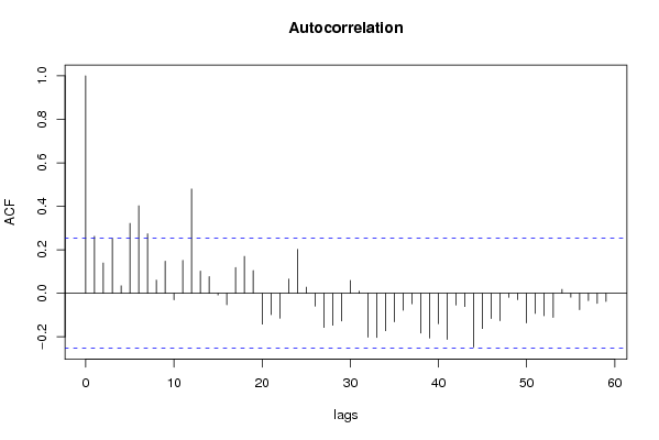
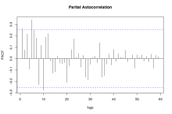
Title produced by software

(Partial) Autocorrelation Function

Date of computation

Mon, 08 Dec 2008 14:18:59 -0700

Cite this page as follows

Statistical Computations at FreeStatistics.org, Office for Research Development and Education, URL https://freestatistics.org/blog/index.php?v=date/2008/Dec/08/t1228771169u17z8ao0d7aol03.htm/, Retrieved Thu, 16 May 2024 16:34:51 +0000

Statistical Computations at FreeStatistics.org, Office for Research Development and Education, URL https://freestatistics.org/blog/index.php?pk=31049, Retrieved Thu, 16 May 2024 16:34:51 +0000

QR Codes:

Paste this QR Code to cite your computation.

Original text written by user:

IsPrivate?

No (this computation is public)

User-defined keywords

Estimated Impact

175

Family? (F = Feedback message, R = changed R code, M = changed R Module, P = changed Parameters, D = changed Data)

F     [(Partial) Autocorrelation Function] [Unemployment - St...] [2008-12-08 17:24:07] [57850c80fd59ccfb28f882be994e814e]
F   P   [(Partial) Autocorrelation Function] [Unemployment - St...] [2008-12-08 18:00:18] [57850c80fd59ccfb28f882be994e814e]
F    D      [(Partial) Autocorrelation Function] [] [2008-12-08 21:18:59] [6d40a467de0f28bd2350f82ac9522c51] [Current]

Feedback Forum

2008-12-14 08:47:19 [Kristof Van Esbroeck] [reply] 
Variance reduction matrix 
 
http://www.freestatistics.org/blog/index.php?v=date/2008/Dec/14/t1229240745tj03ke3f5u90k7i.htm 
 
We noteren de kleinste waarde 795.483036989776 waar d = 1 en D = 1, dit wil zeggen dat we één maal gewoon en één maal seizonaal moeten differentiëren om de datareeks stationair te maken. 
 
Autocorrelation function 
 
http://www.freestatistics.org/blog/index.php?v=date/2008/Dec/14/t1229240981bunrvmi07orhxzk.htm 
 
Wanneer we de grafiek analyseren merken we duidelijk een lange termijn trend op. Deze werken we weg door de parameters correct aan te passen. 
 
http://www.freestatistics.org/blog/index.php?v=date/2008/Dec/14/t122924127550xavkph4wzg4t3.htm 
 
Op deze grafiek is de trend verdwenen, we merken enkel nog dat de datareeks gevoelig is aan de economische conjunctuur. 
 
Cumulative periodogram 
 
http://www.freestatistics.org/blog/index.php?v=date/2008/Dec/14/t1229241558k1rb20mpetsflgm.htm 
 
De parameters werden correct ingegeven zoals in de Variance reduction matrix reeds werd gesteld. We voeren d = 1 en D = 1 in om een berekening te maken. 
2008-12-15 08:25:11 [Nathalie Koulouris] [reply] 
De student had inderdaad hier eerst de VRM moeten berekenen. Hij heeft nu zijn verbetering correct uitgevoerd

Post a new message

Dataseries X:

Download CSV

Histogram

Boxplots

Summary of computational transaction
Raw Input	view raw input (R code)
Raw Output	view raw output of R engine
Computing time	0 seconds
R Server	'Gwilym Jenkins' @ 72.249.127.135

\begin{tabular}{lllllllll}
\hline
Summary of computational transaction \tabularnewline
Raw Input & view raw input (R code)  \tabularnewline
Raw Output & view raw output of R engine  \tabularnewline
Computing time & 0 seconds \tabularnewline
R Server & 'Gwilym Jenkins' @ 72.249.127.135 \tabularnewline
\hline
\end{tabular}
%Source: https://freestatistics.org/blog/index.php?pk=31049&T=0

[TABLE]
[ROW][C]Summary of computational transaction[/C][/ROW]
[ROW][C]Raw Input[/C][C]view raw input (R code) [/C][/ROW]
[ROW][C]Raw Output[/C][C]view raw output of R engine [/C][/ROW]
[ROW][C]Computing time[/C][C]0 seconds[/C][/ROW]
[ROW][C]R Server[/C][C]'Gwilym Jenkins' @ 72.249.127.135[/C][/ROW]
[/TABLE]
Source: https://freestatistics.org/blog/index.php?pk=31049&T=0

Globally Unique Identifier (entire table): ba.freestatistics.org/blog/index.php?pk=31049&T=0

As an alternative you can also use a QR Code:

The GUIDs for individual cells are displayed in the table below:

Summary of computational transaction
Raw Input	view raw input (R code)
Raw Output	view raw output of R engine
Computing time	0 seconds
R Server	'Gwilym Jenkins' @ 72.249.127.135

Autocorrelation Function
Time lag k	ACF(k)	T-STAT	P-value
1	0.262173	2.0308	0.023358
2	0.139385	1.0797	0.142305
3	0.252716	1.9575	0.027471
4	0.034428	0.2667	0.395317
5	0.321785	2.4925	0.007731
6	0.402764	3.1198	0.00139
7	0.273528	2.1187	0.019131
8	0.060745	0.4705	0.319842
9	0.147484	1.1424	0.128912
10	-0.030195	-0.2339	0.407934
11	0.15129	1.1719	0.122937
12	0.479581	3.7148	0.000224
13	0.102247	0.792	0.21574
14	0.076573	0.5931	0.277662
15	-0.007718	-0.0598	0.476263
16	-0.052931	-0.41	0.341632
17	0.118918	0.9211	0.180334
18	0.169845	1.3156	0.096655
19	0.104395	0.8086	0.210958
20	-0.142179	-1.1013	0.137579
21	-0.098139	-0.7602	0.225061
22	-0.11455	-0.8873	0.18923
23	0.06579	0.5096	0.306098
24	0.201897	1.5639	0.061552
25	0.02843	0.2202	0.413224
26	-0.058917	-0.4564	0.324887
27	-0.156952	-1.2157	0.114422
28	-0.146877	-1.1377	0.129883
29	-0.127512	-0.9877	0.163633
30	0.059106	0.4578	0.324364
31	0.009921	0.0769	0.469499
32	-0.202069	-1.5652	0.061395
33	-0.203445	-1.5759	0.060157
34	-0.17245	-1.3358	0.093331
35	-0.13145	-1.0182	0.156334
36	-0.07806	-0.6046	0.273846
37	-0.048101	-0.3726	0.355384
38	-0.183298	-1.4198	0.080418
39	-0.205594	-1.5925	0.058261
40	-0.139773	-1.0827	0.141641
41	-0.212042	-1.6425	0.052862
42	-0.054083	-0.4189	0.338384
43	-0.060876	-0.4715	0.319481
44	-0.247402	-1.9164	0.030043
45	-0.162222	-1.2566	0.10689
46	-0.116048	-0.8989	0.186149
47	-0.126286	-0.9782	0.165949
48	-0.018508	-0.1434	0.443243
49	-0.029286	-0.2268	0.410656
50	-0.136527	-1.0575	0.147253
51	-0.092735	-0.7183	0.237672
52	-0.103138	-0.7989	0.213748
53	-0.110982	-0.8597	0.196698
54	0.018343	0.1421	0.443745
55	-0.017742	-0.1374	0.445577
56	-0.075377	-0.5839	0.28075
57	-0.033646	-0.2606	0.397638
58	-0.046351	-0.359	0.360416
59	-0.037882	-0.2934	0.385103
60	NA	NA	NA

\begin{tabular}{lllllllll}
\hline
Autocorrelation Function \tabularnewline
Time lag k & ACF(k) & T-STAT & P-value \tabularnewline
1 & 0.262173 & 2.0308 & 0.023358 \tabularnewline
2 & 0.139385 & 1.0797 & 0.142305 \tabularnewline
3 & 0.252716 & 1.9575 & 0.027471 \tabularnewline
4 & 0.034428 & 0.2667 & 0.395317 \tabularnewline
5 & 0.321785 & 2.4925 & 0.007731 \tabularnewline
6 & 0.402764 & 3.1198 & 0.00139 \tabularnewline
7 & 0.273528 & 2.1187 & 0.019131 \tabularnewline
8 & 0.060745 & 0.4705 & 0.319842 \tabularnewline
9 & 0.147484 & 1.1424 & 0.128912 \tabularnewline
10 & -0.030195 & -0.2339 & 0.407934 \tabularnewline
11 & 0.15129 & 1.1719 & 0.122937 \tabularnewline
12 & 0.479581 & 3.7148 & 0.000224 \tabularnewline
13 & 0.102247 & 0.792 & 0.21574 \tabularnewline
14 & 0.076573 & 0.5931 & 0.277662 \tabularnewline
15 & -0.007718 & -0.0598 & 0.476263 \tabularnewline
16 & -0.052931 & -0.41 & 0.341632 \tabularnewline
17 & 0.118918 & 0.9211 & 0.180334 \tabularnewline
18 & 0.169845 & 1.3156 & 0.096655 \tabularnewline
19 & 0.104395 & 0.8086 & 0.210958 \tabularnewline
20 & -0.142179 & -1.1013 & 0.137579 \tabularnewline
21 & -0.098139 & -0.7602 & 0.225061 \tabularnewline
22 & -0.11455 & -0.8873 & 0.18923 \tabularnewline
23 & 0.06579 & 0.5096 & 0.306098 \tabularnewline
24 & 0.201897 & 1.5639 & 0.061552 \tabularnewline
25 & 0.02843 & 0.2202 & 0.413224 \tabularnewline
26 & -0.058917 & -0.4564 & 0.324887 \tabularnewline
27 & -0.156952 & -1.2157 & 0.114422 \tabularnewline
28 & -0.146877 & -1.1377 & 0.129883 \tabularnewline
29 & -0.127512 & -0.9877 & 0.163633 \tabularnewline
30 & 0.059106 & 0.4578 & 0.324364 \tabularnewline
31 & 0.009921 & 0.0769 & 0.469499 \tabularnewline
32 & -0.202069 & -1.5652 & 0.061395 \tabularnewline
33 & -0.203445 & -1.5759 & 0.060157 \tabularnewline
34 & -0.17245 & -1.3358 & 0.093331 \tabularnewline
35 & -0.13145 & -1.0182 & 0.156334 \tabularnewline
36 & -0.07806 & -0.6046 & 0.273846 \tabularnewline
37 & -0.048101 & -0.3726 & 0.355384 \tabularnewline
38 & -0.183298 & -1.4198 & 0.080418 \tabularnewline
39 & -0.205594 & -1.5925 & 0.058261 \tabularnewline
40 & -0.139773 & -1.0827 & 0.141641 \tabularnewline
41 & -0.212042 & -1.6425 & 0.052862 \tabularnewline
42 & -0.054083 & -0.4189 & 0.338384 \tabularnewline
43 & -0.060876 & -0.4715 & 0.319481 \tabularnewline
44 & -0.247402 & -1.9164 & 0.030043 \tabularnewline
45 & -0.162222 & -1.2566 & 0.10689 \tabularnewline
46 & -0.116048 & -0.8989 & 0.186149 \tabularnewline
47 & -0.126286 & -0.9782 & 0.165949 \tabularnewline
48 & -0.018508 & -0.1434 & 0.443243 \tabularnewline
49 & -0.029286 & -0.2268 & 0.410656 \tabularnewline
50 & -0.136527 & -1.0575 & 0.147253 \tabularnewline
51 & -0.092735 & -0.7183 & 0.237672 \tabularnewline
52 & -0.103138 & -0.7989 & 0.213748 \tabularnewline
53 & -0.110982 & -0.8597 & 0.196698 \tabularnewline
54 & 0.018343 & 0.1421 & 0.443745 \tabularnewline
55 & -0.017742 & -0.1374 & 0.445577 \tabularnewline
56 & -0.075377 & -0.5839 & 0.28075 \tabularnewline
57 & -0.033646 & -0.2606 & 0.397638 \tabularnewline
58 & -0.046351 & -0.359 & 0.360416 \tabularnewline
59 & -0.037882 & -0.2934 & 0.385103 \tabularnewline
60 & NA & NA & NA \tabularnewline
\hline
\end{tabular}
%Source: https://freestatistics.org/blog/index.php?pk=31049&T=1

[TABLE]
[ROW][C]Autocorrelation Function[/C][/ROW]
[ROW][C]Time lag k[/C][C]ACF(k)[/C][C]T-STAT[/C][C]P-value[/C][/ROW]
[ROW][C]1[/C][C]0.262173[/C][C]2.0308[/C][C]0.023358[/C][/ROW]
[ROW][C]2[/C][C]0.139385[/C][C]1.0797[/C][C]0.142305[/C][/ROW]
[ROW][C]3[/C][C]0.252716[/C][C]1.9575[/C][C]0.027471[/C][/ROW]
[ROW][C]4[/C][C]0.034428[/C][C]0.2667[/C][C]0.395317[/C][/ROW]
[ROW][C]5[/C][C]0.321785[/C][C]2.4925[/C][C]0.007731[/C][/ROW]
[ROW][C]6[/C][C]0.402764[/C][C]3.1198[/C][C]0.00139[/C][/ROW]
[ROW][C]7[/C][C]0.273528[/C][C]2.1187[/C][C]0.019131[/C][/ROW]
[ROW][C]8[/C][C]0.060745[/C][C]0.4705[/C][C]0.319842[/C][/ROW]
[ROW][C]9[/C][C]0.147484[/C][C]1.1424[/C][C]0.128912[/C][/ROW]
[ROW][C]10[/C][C]-0.030195[/C][C]-0.2339[/C][C]0.407934[/C][/ROW]
[ROW][C]11[/C][C]0.15129[/C][C]1.1719[/C][C]0.122937[/C][/ROW]
[ROW][C]12[/C][C]0.479581[/C][C]3.7148[/C][C]0.000224[/C][/ROW]
[ROW][C]13[/C][C]0.102247[/C][C]0.792[/C][C]0.21574[/C][/ROW]
[ROW][C]14[/C][C]0.076573[/C][C]0.5931[/C][C]0.277662[/C][/ROW]
[ROW][C]15[/C][C]-0.007718[/C][C]-0.0598[/C][C]0.476263[/C][/ROW]
[ROW][C]16[/C][C]-0.052931[/C][C]-0.41[/C][C]0.341632[/C][/ROW]
[ROW][C]17[/C][C]0.118918[/C][C]0.9211[/C][C]0.180334[/C][/ROW]
[ROW][C]18[/C][C]0.169845[/C][C]1.3156[/C][C]0.096655[/C][/ROW]
[ROW][C]19[/C][C]0.104395[/C][C]0.8086[/C][C]0.210958[/C][/ROW]
[ROW][C]20[/C][C]-0.142179[/C][C]-1.1013[/C][C]0.137579[/C][/ROW]
[ROW][C]21[/C][C]-0.098139[/C][C]-0.7602[/C][C]0.225061[/C][/ROW]
[ROW][C]22[/C][C]-0.11455[/C][C]-0.8873[/C][C]0.18923[/C][/ROW]
[ROW][C]23[/C][C]0.06579[/C][C]0.5096[/C][C]0.306098[/C][/ROW]
[ROW][C]24[/C][C]0.201897[/C][C]1.5639[/C][C]0.061552[/C][/ROW]
[ROW][C]25[/C][C]0.02843[/C][C]0.2202[/C][C]0.413224[/C][/ROW]
[ROW][C]26[/C][C]-0.058917[/C][C]-0.4564[/C][C]0.324887[/C][/ROW]
[ROW][C]27[/C][C]-0.156952[/C][C]-1.2157[/C][C]0.114422[/C][/ROW]
[ROW][C]28[/C][C]-0.146877[/C][C]-1.1377[/C][C]0.129883[/C][/ROW]
[ROW][C]29[/C][C]-0.127512[/C][C]-0.9877[/C][C]0.163633[/C][/ROW]
[ROW][C]30[/C][C]0.059106[/C][C]0.4578[/C][C]0.324364[/C][/ROW]
[ROW][C]31[/C][C]0.009921[/C][C]0.0769[/C][C]0.469499[/C][/ROW]
[ROW][C]32[/C][C]-0.202069[/C][C]-1.5652[/C][C]0.061395[/C][/ROW]
[ROW][C]33[/C][C]-0.203445[/C][C]-1.5759[/C][C]0.060157[/C][/ROW]
[ROW][C]34[/C][C]-0.17245[/C][C]-1.3358[/C][C]0.093331[/C][/ROW]
[ROW][C]35[/C][C]-0.13145[/C][C]-1.0182[/C][C]0.156334[/C][/ROW]
[ROW][C]36[/C][C]-0.07806[/C][C]-0.6046[/C][C]0.273846[/C][/ROW]
[ROW][C]37[/C][C]-0.048101[/C][C]-0.3726[/C][C]0.355384[/C][/ROW]
[ROW][C]38[/C][C]-0.183298[/C][C]-1.4198[/C][C]0.080418[/C][/ROW]
[ROW][C]39[/C][C]-0.205594[/C][C]-1.5925[/C][C]0.058261[/C][/ROW]
[ROW][C]40[/C][C]-0.139773[/C][C]-1.0827[/C][C]0.141641[/C][/ROW]
[ROW][C]41[/C][C]-0.212042[/C][C]-1.6425[/C][C]0.052862[/C][/ROW]
[ROW][C]42[/C][C]-0.054083[/C][C]-0.4189[/C][C]0.338384[/C][/ROW]
[ROW][C]43[/C][C]-0.060876[/C][C]-0.4715[/C][C]0.319481[/C][/ROW]
[ROW][C]44[/C][C]-0.247402[/C][C]-1.9164[/C][C]0.030043[/C][/ROW]
[ROW][C]45[/C][C]-0.162222[/C][C]-1.2566[/C][C]0.10689[/C][/ROW]
[ROW][C]46[/C][C]-0.116048[/C][C]-0.8989[/C][C]0.186149[/C][/ROW]
[ROW][C]47[/C][C]-0.126286[/C][C]-0.9782[/C][C]0.165949[/C][/ROW]
[ROW][C]48[/C][C]-0.018508[/C][C]-0.1434[/C][C]0.443243[/C][/ROW]
[ROW][C]49[/C][C]-0.029286[/C][C]-0.2268[/C][C]0.410656[/C][/ROW]
[ROW][C]50[/C][C]-0.136527[/C][C]-1.0575[/C][C]0.147253[/C][/ROW]
[ROW][C]51[/C][C]-0.092735[/C][C]-0.7183[/C][C]0.237672[/C][/ROW]
[ROW][C]52[/C][C]-0.103138[/C][C]-0.7989[/C][C]0.213748[/C][/ROW]
[ROW][C]53[/C][C]-0.110982[/C][C]-0.8597[/C][C]0.196698[/C][/ROW]
[ROW][C]54[/C][C]0.018343[/C][C]0.1421[/C][C]0.443745[/C][/ROW]
[ROW][C]55[/C][C]-0.017742[/C][C]-0.1374[/C][C]0.445577[/C][/ROW]
[ROW][C]56[/C][C]-0.075377[/C][C]-0.5839[/C][C]0.28075[/C][/ROW]
[ROW][C]57[/C][C]-0.033646[/C][C]-0.2606[/C][C]0.397638[/C][/ROW]
[ROW][C]58[/C][C]-0.046351[/C][C]-0.359[/C][C]0.360416[/C][/ROW]
[ROW][C]59[/C][C]-0.037882[/C][C]-0.2934[/C][C]0.385103[/C][/ROW]
[ROW][C]60[/C][C]NA[/C][C]NA[/C][C]NA[/C][/ROW]
[/TABLE]
Source: https://freestatistics.org/blog/index.php?pk=31049&T=1

Globally Unique Identifier (entire table): ba.freestatistics.org/blog/index.php?pk=31049&T=1

As an alternative you can also use a QR Code:

The GUIDs for individual cells are displayed in the table below:

Autocorrelation Function
Time lag k	ACF(k)	T-STAT	P-value
1	0.262173	2.0308	0.023358
2	0.139385	1.0797	0.142305
3	0.252716	1.9575	0.027471
4	0.034428	0.2667	0.395317
5	0.321785	2.4925	0.007731
6	0.402764	3.1198	0.00139
7	0.273528	2.1187	0.019131
8	0.060745	0.4705	0.319842
9	0.147484	1.1424	0.128912
10	-0.030195	-0.2339	0.407934
11	0.15129	1.1719	0.122937
12	0.479581	3.7148	0.000224
13	0.102247	0.792	0.21574
14	0.076573	0.5931	0.277662
15	-0.007718	-0.0598	0.476263
16	-0.052931	-0.41	0.341632
17	0.118918	0.9211	0.180334
18	0.169845	1.3156	0.096655
19	0.104395	0.8086	0.210958
20	-0.142179	-1.1013	0.137579
21	-0.098139	-0.7602	0.225061
22	-0.11455	-0.8873	0.18923
23	0.06579	0.5096	0.306098
24	0.201897	1.5639	0.061552
25	0.02843	0.2202	0.413224
26	-0.058917	-0.4564	0.324887
27	-0.156952	-1.2157	0.114422
28	-0.146877	-1.1377	0.129883
29	-0.127512	-0.9877	0.163633
30	0.059106	0.4578	0.324364
31	0.009921	0.0769	0.469499
32	-0.202069	-1.5652	0.061395
33	-0.203445	-1.5759	0.060157
34	-0.17245	-1.3358	0.093331
35	-0.13145	-1.0182	0.156334
36	-0.07806	-0.6046	0.273846
37	-0.048101	-0.3726	0.355384
38	-0.183298	-1.4198	0.080418
39	-0.205594	-1.5925	0.058261
40	-0.139773	-1.0827	0.141641
41	-0.212042	-1.6425	0.052862
42	-0.054083	-0.4189	0.338384
43	-0.060876	-0.4715	0.319481
44	-0.247402	-1.9164	0.030043
45	-0.162222	-1.2566	0.10689
46	-0.116048	-0.8989	0.186149
47	-0.126286	-0.9782	0.165949
48	-0.018508	-0.1434	0.443243
49	-0.029286	-0.2268	0.410656
50	-0.136527	-1.0575	0.147253
51	-0.092735	-0.7183	0.237672
52	-0.103138	-0.7989	0.213748
53	-0.110982	-0.8597	0.196698
54	0.018343	0.1421	0.443745
55	-0.017742	-0.1374	0.445577
56	-0.075377	-0.5839	0.28075
57	-0.033646	-0.2606	0.397638
58	-0.046351	-0.359	0.360416
59	-0.037882	-0.2934	0.385103
60	NA	NA	NA

Partial Autocorrelation Function
Time lag k	PACF(k)	T-STAT	P-value
1	0.262173	2.0308	0.023358
2	0.075865	0.5876	0.279487
3	0.214984	1.6653	0.050537
4	-0.093257	-0.7224	0.236437
5	0.340737	2.6393	0.005285
6	0.249655	1.9338	0.028928
7	0.18105	1.4024	0.082973
8	-0.227768	-1.7643	0.041387
9	0.117189	0.9077	0.183824
10	-0.277117	-2.1465	0.017941
11	0.188131	1.4573	0.075129
12	0.218469	1.6923	0.047893
13	-0.01971	-0.1527	0.439585
14	-0.127906	-0.9908	0.162891
15	-0.117372	-0.9092	0.183451
16	0.023837	0.1846	0.427068
17	-0.038429	-0.2977	0.383493
18	-0.048016	-0.3719	0.355628
19	-0.035782	-0.2772	0.391303
20	-0.208624	-1.616	0.055671
21	-0.06408	-0.4964	0.310727
22	0.078373	0.6071	0.273045
23	0.173482	1.3438	0.092039
24	0.010859	0.0841	0.466623
25	0.046414	0.3595	0.360234
26	-0.075035	-0.5812	0.281636
27	0.028335	0.2195	0.413511
28	-0.161772	-1.2531	0.107519
29	-0.185226	-1.4348	0.078275
30	-0.051527	-0.3991	0.34561
31	0.010753	0.0833	0.466949
32	0.023332	0.1807	0.428594
33	-0.034236	-0.2652	0.395885
34	0.138657	1.074	0.143554
35	-0.163148	-1.2637	0.105606
36	-0.149067	-1.1547	0.126402
37	-0.05001	-0.3874	0.349925
38	0.04252	0.3294	0.371516
39	-0.057143	-0.4426	0.329814
40	0.080397	0.6228	0.267903
41	-0.026385	-0.2044	0.419375
42	0.044212	0.3425	0.366599
43	0.012674	0.0982	0.46106
44	0.010931	0.0847	0.466402
45	0.072887	0.5646	0.287231
46	-0.026771	-0.2074	0.418211
47	-0.003625	-0.0281	0.488846
48	0.033743	0.2614	0.397351
49	-0.085592	-0.663	0.254937
50	0.034034	0.2636	0.396485
51	0.011391	0.0882	0.464993
52	0.033178	0.257	0.39903
53	-0.022717	-0.176	0.430456
54	0.018752	0.1453	0.442498
55	-0.02896	-0.2243	0.411634
56	0.040752	0.3157	0.376676
57	-0.084816	-0.657	0.256853
58	0.029995	0.2323	0.408533
59	0.017403	0.1348	0.446611
60	NA	NA	NA

\begin{tabular}{lllllllll}
\hline
Partial Autocorrelation Function \tabularnewline
Time lag k & PACF(k) & T-STAT & P-value \tabularnewline
1 & 0.262173 & 2.0308 & 0.023358 \tabularnewline
2 & 0.075865 & 0.5876 & 0.279487 \tabularnewline
3 & 0.214984 & 1.6653 & 0.050537 \tabularnewline
4 & -0.093257 & -0.7224 & 0.236437 \tabularnewline
5 & 0.340737 & 2.6393 & 0.005285 \tabularnewline
6 & 0.249655 & 1.9338 & 0.028928 \tabularnewline
7 & 0.18105 & 1.4024 & 0.082973 \tabularnewline
8 & -0.227768 & -1.7643 & 0.041387 \tabularnewline
9 & 0.117189 & 0.9077 & 0.183824 \tabularnewline
10 & -0.277117 & -2.1465 & 0.017941 \tabularnewline
11 & 0.188131 & 1.4573 & 0.075129 \tabularnewline
12 & 0.218469 & 1.6923 & 0.047893 \tabularnewline
13 & -0.01971 & -0.1527 & 0.439585 \tabularnewline
14 & -0.127906 & -0.9908 & 0.162891 \tabularnewline
15 & -0.117372 & -0.9092 & 0.183451 \tabularnewline
16 & 0.023837 & 0.1846 & 0.427068 \tabularnewline
17 & -0.038429 & -0.2977 & 0.383493 \tabularnewline
18 & -0.048016 & -0.3719 & 0.355628 \tabularnewline
19 & -0.035782 & -0.2772 & 0.391303 \tabularnewline
20 & -0.208624 & -1.616 & 0.055671 \tabularnewline
21 & -0.06408 & -0.4964 & 0.310727 \tabularnewline
22 & 0.078373 & 0.6071 & 0.273045 \tabularnewline
23 & 0.173482 & 1.3438 & 0.092039 \tabularnewline
24 & 0.010859 & 0.0841 & 0.466623 \tabularnewline
25 & 0.046414 & 0.3595 & 0.360234 \tabularnewline
26 & -0.075035 & -0.5812 & 0.281636 \tabularnewline
27 & 0.028335 & 0.2195 & 0.413511 \tabularnewline
28 & -0.161772 & -1.2531 & 0.107519 \tabularnewline
29 & -0.185226 & -1.4348 & 0.078275 \tabularnewline
30 & -0.051527 & -0.3991 & 0.34561 \tabularnewline
31 & 0.010753 & 0.0833 & 0.466949 \tabularnewline
32 & 0.023332 & 0.1807 & 0.428594 \tabularnewline
33 & -0.034236 & -0.2652 & 0.395885 \tabularnewline
34 & 0.138657 & 1.074 & 0.143554 \tabularnewline
35 & -0.163148 & -1.2637 & 0.105606 \tabularnewline
36 & -0.149067 & -1.1547 & 0.126402 \tabularnewline
37 & -0.05001 & -0.3874 & 0.349925 \tabularnewline
38 & 0.04252 & 0.3294 & 0.371516 \tabularnewline
39 & -0.057143 & -0.4426 & 0.329814 \tabularnewline
40 & 0.080397 & 0.6228 & 0.267903 \tabularnewline
41 & -0.026385 & -0.2044 & 0.419375 \tabularnewline
42 & 0.044212 & 0.3425 & 0.366599 \tabularnewline
43 & 0.012674 & 0.0982 & 0.46106 \tabularnewline
44 & 0.010931 & 0.0847 & 0.466402 \tabularnewline
45 & 0.072887 & 0.5646 & 0.287231 \tabularnewline
46 & -0.026771 & -0.2074 & 0.418211 \tabularnewline
47 & -0.003625 & -0.0281 & 0.488846 \tabularnewline
48 & 0.033743 & 0.2614 & 0.397351 \tabularnewline
49 & -0.085592 & -0.663 & 0.254937 \tabularnewline
50 & 0.034034 & 0.2636 & 0.396485 \tabularnewline
51 & 0.011391 & 0.0882 & 0.464993 \tabularnewline
52 & 0.033178 & 0.257 & 0.39903 \tabularnewline
53 & -0.022717 & -0.176 & 0.430456 \tabularnewline
54 & 0.018752 & 0.1453 & 0.442498 \tabularnewline
55 & -0.02896 & -0.2243 & 0.411634 \tabularnewline
56 & 0.040752 & 0.3157 & 0.376676 \tabularnewline
57 & -0.084816 & -0.657 & 0.256853 \tabularnewline
58 & 0.029995 & 0.2323 & 0.408533 \tabularnewline
59 & 0.017403 & 0.1348 & 0.446611 \tabularnewline
60 & NA & NA & NA \tabularnewline
\hline
\end{tabular}
%Source: https://freestatistics.org/blog/index.php?pk=31049&T=2

[TABLE]
[ROW][C]Partial Autocorrelation Function[/C][/ROW]
[ROW][C]Time lag k[/C][C]PACF(k)[/C][C]T-STAT[/C][C]P-value[/C][/ROW]
[ROW][C]1[/C][C]0.262173[/C][C]2.0308[/C][C]0.023358[/C][/ROW]
[ROW][C]2[/C][C]0.075865[/C][C]0.5876[/C][C]0.279487[/C][/ROW]
[ROW][C]3[/C][C]0.214984[/C][C]1.6653[/C][C]0.050537[/C][/ROW]
[ROW][C]4[/C][C]-0.093257[/C][C]-0.7224[/C][C]0.236437[/C][/ROW]
[ROW][C]5[/C][C]0.340737[/C][C]2.6393[/C][C]0.005285[/C][/ROW]
[ROW][C]6[/C][C]0.249655[/C][C]1.9338[/C][C]0.028928[/C][/ROW]
[ROW][C]7[/C][C]0.18105[/C][C]1.4024[/C][C]0.082973[/C][/ROW]
[ROW][C]8[/C][C]-0.227768[/C][C]-1.7643[/C][C]0.041387[/C][/ROW]
[ROW][C]9[/C][C]0.117189[/C][C]0.9077[/C][C]0.183824[/C][/ROW]
[ROW][C]10[/C][C]-0.277117[/C][C]-2.1465[/C][C]0.017941[/C][/ROW]
[ROW][C]11[/C][C]0.188131[/C][C]1.4573[/C][C]0.075129[/C][/ROW]
[ROW][C]12[/C][C]0.218469[/C][C]1.6923[/C][C]0.047893[/C][/ROW]
[ROW][C]13[/C][C]-0.01971[/C][C]-0.1527[/C][C]0.439585[/C][/ROW]
[ROW][C]14[/C][C]-0.127906[/C][C]-0.9908[/C][C]0.162891[/C][/ROW]
[ROW][C]15[/C][C]-0.117372[/C][C]-0.9092[/C][C]0.183451[/C][/ROW]
[ROW][C]16[/C][C]0.023837[/C][C]0.1846[/C][C]0.427068[/C][/ROW]
[ROW][C]17[/C][C]-0.038429[/C][C]-0.2977[/C][C]0.383493[/C][/ROW]
[ROW][C]18[/C][C]-0.048016[/C][C]-0.3719[/C][C]0.355628[/C][/ROW]
[ROW][C]19[/C][C]-0.035782[/C][C]-0.2772[/C][C]0.391303[/C][/ROW]
[ROW][C]20[/C][C]-0.208624[/C][C]-1.616[/C][C]0.055671[/C][/ROW]
[ROW][C]21[/C][C]-0.06408[/C][C]-0.4964[/C][C]0.310727[/C][/ROW]
[ROW][C]22[/C][C]0.078373[/C][C]0.6071[/C][C]0.273045[/C][/ROW]
[ROW][C]23[/C][C]0.173482[/C][C]1.3438[/C][C]0.092039[/C][/ROW]
[ROW][C]24[/C][C]0.010859[/C][C]0.0841[/C][C]0.466623[/C][/ROW]
[ROW][C]25[/C][C]0.046414[/C][C]0.3595[/C][C]0.360234[/C][/ROW]
[ROW][C]26[/C][C]-0.075035[/C][C]-0.5812[/C][C]0.281636[/C][/ROW]
[ROW][C]27[/C][C]0.028335[/C][C]0.2195[/C][C]0.413511[/C][/ROW]
[ROW][C]28[/C][C]-0.161772[/C][C]-1.2531[/C][C]0.107519[/C][/ROW]
[ROW][C]29[/C][C]-0.185226[/C][C]-1.4348[/C][C]0.078275[/C][/ROW]
[ROW][C]30[/C][C]-0.051527[/C][C]-0.3991[/C][C]0.34561[/C][/ROW]
[ROW][C]31[/C][C]0.010753[/C][C]0.0833[/C][C]0.466949[/C][/ROW]
[ROW][C]32[/C][C]0.023332[/C][C]0.1807[/C][C]0.428594[/C][/ROW]
[ROW][C]33[/C][C]-0.034236[/C][C]-0.2652[/C][C]0.395885[/C][/ROW]
[ROW][C]34[/C][C]0.138657[/C][C]1.074[/C][C]0.143554[/C][/ROW]
[ROW][C]35[/C][C]-0.163148[/C][C]-1.2637[/C][C]0.105606[/C][/ROW]
[ROW][C]36[/C][C]-0.149067[/C][C]-1.1547[/C][C]0.126402[/C][/ROW]
[ROW][C]37[/C][C]-0.05001[/C][C]-0.3874[/C][C]0.349925[/C][/ROW]
[ROW][C]38[/C][C]0.04252[/C][C]0.3294[/C][C]0.371516[/C][/ROW]
[ROW][C]39[/C][C]-0.057143[/C][C]-0.4426[/C][C]0.329814[/C][/ROW]
[ROW][C]40[/C][C]0.080397[/C][C]0.6228[/C][C]0.267903[/C][/ROW]
[ROW][C]41[/C][C]-0.026385[/C][C]-0.2044[/C][C]0.419375[/C][/ROW]
[ROW][C]42[/C][C]0.044212[/C][C]0.3425[/C][C]0.366599[/C][/ROW]
[ROW][C]43[/C][C]0.012674[/C][C]0.0982[/C][C]0.46106[/C][/ROW]
[ROW][C]44[/C][C]0.010931[/C][C]0.0847[/C][C]0.466402[/C][/ROW]
[ROW][C]45[/C][C]0.072887[/C][C]0.5646[/C][C]0.287231[/C][/ROW]
[ROW][C]46[/C][C]-0.026771[/C][C]-0.2074[/C][C]0.418211[/C][/ROW]
[ROW][C]47[/C][C]-0.003625[/C][C]-0.0281[/C][C]0.488846[/C][/ROW]
[ROW][C]48[/C][C]0.033743[/C][C]0.2614[/C][C]0.397351[/C][/ROW]
[ROW][C]49[/C][C]-0.085592[/C][C]-0.663[/C][C]0.254937[/C][/ROW]
[ROW][C]50[/C][C]0.034034[/C][C]0.2636[/C][C]0.396485[/C][/ROW]
[ROW][C]51[/C][C]0.011391[/C][C]0.0882[/C][C]0.464993[/C][/ROW]
[ROW][C]52[/C][C]0.033178[/C][C]0.257[/C][C]0.39903[/C][/ROW]
[ROW][C]53[/C][C]-0.022717[/C][C]-0.176[/C][C]0.430456[/C][/ROW]
[ROW][C]54[/C][C]0.018752[/C][C]0.1453[/C][C]0.442498[/C][/ROW]
[ROW][C]55[/C][C]-0.02896[/C][C]-0.2243[/C][C]0.411634[/C][/ROW]
[ROW][C]56[/C][C]0.040752[/C][C]0.3157[/C][C]0.376676[/C][/ROW]
[ROW][C]57[/C][C]-0.084816[/C][C]-0.657[/C][C]0.256853[/C][/ROW]
[ROW][C]58[/C][C]0.029995[/C][C]0.2323[/C][C]0.408533[/C][/ROW]
[ROW][C]59[/C][C]0.017403[/C][C]0.1348[/C][C]0.446611[/C][/ROW]
[ROW][C]60[/C][C]NA[/C][C]NA[/C][C]NA[/C][/ROW]
[/TABLE]
Source: https://freestatistics.org/blog/index.php?pk=31049&T=2

Globally Unique Identifier (entire table): ba.freestatistics.org/blog/index.php?pk=31049&T=2

As an alternative you can also use a QR Code:

The GUIDs for individual cells are displayed in the table below:

Partial Autocorrelation Function
Time lag k	PACF(k)	T-STAT	P-value
1	0.262173	2.0308	0.023358
2	0.075865	0.5876	0.279487
3	0.214984	1.6653	0.050537
4	-0.093257	-0.7224	0.236437
5	0.340737	2.6393	0.005285
6	0.249655	1.9338	0.028928
7	0.18105	1.4024	0.082973
8	-0.227768	-1.7643	0.041387
9	0.117189	0.9077	0.183824
10	-0.277117	-2.1465	0.017941
11	0.188131	1.4573	0.075129
12	0.218469	1.6923	0.047893
13	-0.01971	-0.1527	0.439585
14	-0.127906	-0.9908	0.162891
15	-0.117372	-0.9092	0.183451
16	0.023837	0.1846	0.427068
17	-0.038429	-0.2977	0.383493
18	-0.048016	-0.3719	0.355628
19	-0.035782	-0.2772	0.391303
20	-0.208624	-1.616	0.055671
21	-0.06408	-0.4964	0.310727
22	0.078373	0.6071	0.273045
23	0.173482	1.3438	0.092039
24	0.010859	0.0841	0.466623
25	0.046414	0.3595	0.360234
26	-0.075035	-0.5812	0.281636
27	0.028335	0.2195	0.413511
28	-0.161772	-1.2531	0.107519
29	-0.185226	-1.4348	0.078275
30	-0.051527	-0.3991	0.34561
31	0.010753	0.0833	0.466949
32	0.023332	0.1807	0.428594
33	-0.034236	-0.2652	0.395885
34	0.138657	1.074	0.143554
35	-0.163148	-1.2637	0.105606
36	-0.149067	-1.1547	0.126402
37	-0.05001	-0.3874	0.349925
38	0.04252	0.3294	0.371516
39	-0.057143	-0.4426	0.329814
40	0.080397	0.6228	0.267903
41	-0.026385	-0.2044	0.419375
42	0.044212	0.3425	0.366599
43	0.012674	0.0982	0.46106
44	0.010931	0.0847	0.466402
45	0.072887	0.5646	0.287231
46	-0.026771	-0.2074	0.418211
47	-0.003625	-0.0281	0.488846
48	0.033743	0.2614	0.397351
49	-0.085592	-0.663	0.254937
50	0.034034	0.2636	0.396485
51	0.011391	0.0882	0.464993
52	0.033178	0.257	0.39903
53	-0.022717	-0.176	0.430456
54	0.018752	0.1453	0.442498
55	-0.02896	-0.2243	0.411634
56	0.040752	0.3157	0.376676
57	-0.084816	-0.657	0.256853
58	0.029995	0.2323	0.408533
59	0.017403	0.1348	0.446611
60	NA	NA	NA

Figure 1

PNG link

Postscript link

PDF link

Figure 2

PNG link

Postscript link

PDF link

Parameters (Session):

par1 = 60 ; par2 = 1 ; par3 = 0 ; par4 = 0 ; par5 = 12 ;

Parameters (R input):

par1 = 60 ; par2 = 1 ; par3 = 0 ; par4 = 0 ; par5 = 12 ;

R code (references can be found in the software module):

if (par1 == 'Default') {
par1 = 10*log10(length(x))
} else {
par1 <- as.numeric(par1)
}
par2 <- as.numeric(par2)
par3 <- as.numeric(par3)
par4 <- as.numeric(par4)
par5 <- as.numeric(par5)
if (par2 == 0) {
x <- log(x)
} else {
x <- (x ^ par2 - 1) / par2
}
if (par3 > 0) x <- diff(x,lag=1,difference=par3)
if (par4 > 0) x <- diff(x,lag=par5,difference=par4)
bitmap(file='pic1.png')
racf <- acf(x,par1,main='Autocorrelation',xlab='lags',ylab='ACF')
dev.off()
bitmap(file='pic2.png')
rpacf <- pacf(x,par1,main='Partial Autocorrelation',xlab='lags',ylab='PACF')
dev.off()
(myacf <- c(racf$acf))
(mypacf <- c(rpacf$acf))
lengthx <- length(x)
sqrtn <- sqrt(lengthx)
load(file='createtable')
a<-table.start()
a<-table.row.start(a)
a<-table.element(a,'Autocorrelation Function',4,TRUE)
a<-table.row.end(a)
a<-table.row.start(a)
a<-table.element(a,'Time lag k',header=TRUE)
a<-table.element(a,hyperlink('basics.htm','ACF(k)','click here for more information about the Autocorrelation Function'),header=TRUE)
a<-table.element(a,'T-STAT',header=TRUE)
a<-table.element(a,'P-value',header=TRUE)
a<-table.row.end(a)
for (i in 2:(par1+1)) {
a<-table.row.start(a)
a<-table.element(a,i-1,header=TRUE)
a<-table.element(a,round(myacf[i],6))
mytstat <- myacf[i]*sqrtn
a<-table.element(a,round(mytstat,4))
a<-table.element(a,round(1-pt(abs(mytstat),lengthx),6))
a<-table.row.end(a)
}
a<-table.end(a)
table.save(a,file='mytable.tab')
a<-table.start()
a<-table.row.start(a)
a<-table.element(a,'Partial Autocorrelation Function',4,TRUE)
a<-table.row.end(a)
a<-table.row.start(a)
a<-table.element(a,'Time lag k',header=TRUE)
a<-table.element(a,hyperlink('basics.htm','PACF(k)','click here for more information about the Partial Autocorrelation Function'),header=TRUE)
a<-table.element(a,'T-STAT',header=TRUE)
a<-table.element(a,'P-value',header=TRUE)
a<-table.row.end(a)
for (i in 1:par1) {
a<-table.row.start(a)
a<-table.element(a,i,header=TRUE)
a<-table.element(a,round(mypacf[i],6))
mytstat <- mypacf[i]*sqrtn
a<-table.element(a,round(mytstat,4))
a<-table.element(a,round(1-pt(abs(mytstat),lengthx),6))
a<-table.row.end(a)
}
a<-table.end(a)
table.save(a,file='mytable1.tab')

Free Statistics

Description of Statistical Computation

Tree of Dependent Computations

Dataset

Tables (Output of Computation)

Figures (Output of Computation)

Input Parameters & R Code