Free Statistics
of Irreproducible Research!
Description of Statistical Computation | |||||||||||||||||||||||||||||||||||||||||||||||||||||||||||||||||||||||||||||||||||||||||||||||||||||||||||||||||||||||||||||||||||||||||
|---|---|---|---|---|---|---|---|---|---|---|---|---|---|---|---|---|---|---|---|---|---|---|---|---|---|---|---|---|---|---|---|---|---|---|---|---|---|---|---|---|---|---|---|---|---|---|---|---|---|---|---|---|---|---|---|---|---|---|---|---|---|---|---|---|---|---|---|---|---|---|---|---|---|---|---|---|---|---|---|---|---|---|---|---|---|---|---|---|---|---|---|---|---|---|---|---|---|---|---|---|---|---|---|---|---|---|---|---|---|---|---|---|---|---|---|---|---|---|---|---|---|---|---|---|---|---|---|---|---|---|---|---|---|---|---|---|---|
| Author's title | |||||||||||||||||||||||||||||||||||||||||||||||||||||||||||||||||||||||||||||||||||||||||||||||||||||||||||||||||||||||||||||||||||||||||
| Author | *The author of this computation has been verified* | ||||||||||||||||||||||||||||||||||||||||||||||||||||||||||||||||||||||||||||||||||||||||||||||||||||||||||||||||||||||||||||||||||||||||
| R Software Module | rwasp_smp.wasp | ||||||||||||||||||||||||||||||||||||||||||||||||||||||||||||||||||||||||||||||||||||||||||||||||||||||||||||||||||||||||||||||||||||||||
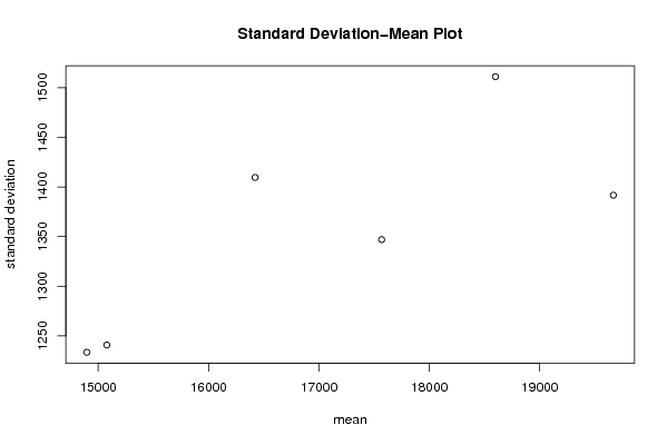
| Title produced by software | Standard Deviation-Mean Plot | ||||||||||||||||||||||||||||||||||||||||||||||||||||||||||||||||||||||||||||||||||||||||||||||||||||||||||||||||||||||||||||||||||||||||
| Date of computation | Mon, 08 Dec 2008 13:09:35 -0700 | ||||||||||||||||||||||||||||||||||||||||||||||||||||||||||||||||||||||||||||||||||||||||||||||||||||||||||||||||||||||||||||||||||||||||
| Cite this page as follows | Statistical Computations at FreeStatistics.org, Office for Research Development and Education, URL https://freestatistics.org/blog/index.php?v=date/2008/Dec/08/t1228767044pedpvshq31jd7fs.htm/, Retrieved Thu, 16 May 2024 18:03:38 +0000 | ||||||||||||||||||||||||||||||||||||||||||||||||||||||||||||||||||||||||||||||||||||||||||||||||||||||||||||||||||||||||||||||||||||||||
| Statistical Computations at FreeStatistics.org, Office for Research Development and Education, URL https://freestatistics.org/blog/index.php?pk=30915, Retrieved Thu, 16 May 2024 18:03:38 +0000 | |||||||||||||||||||||||||||||||||||||||||||||||||||||||||||||||||||||||||||||||||||||||||||||||||||||||||||||||||||||||||||||||||||||||||
| QR Codes: | |||||||||||||||||||||||||||||||||||||||||||||||||||||||||||||||||||||||||||||||||||||||||||||||||||||||||||||||||||||||||||||||||||||||||
|
| |||||||||||||||||||||||||||||||||||||||||||||||||||||||||||||||||||||||||||||||||||||||||||||||||||||||||||||||||||||||||||||||||||||||||
| Original text written by user: | |||||||||||||||||||||||||||||||||||||||||||||||||||||||||||||||||||||||||||||||||||||||||||||||||||||||||||||||||||||||||||||||||||||||||
| IsPrivate? | No (this computation is public) | ||||||||||||||||||||||||||||||||||||||||||||||||||||||||||||||||||||||||||||||||||||||||||||||||||||||||||||||||||||||||||||||||||||||||
| User-defined keywords | |||||||||||||||||||||||||||||||||||||||||||||||||||||||||||||||||||||||||||||||||||||||||||||||||||||||||||||||||||||||||||||||||||||||||
| Estimated Impact | 242 | ||||||||||||||||||||||||||||||||||||||||||||||||||||||||||||||||||||||||||||||||||||||||||||||||||||||||||||||||||||||||||||||||||||||||
Tree of Dependent Computations | |||||||||||||||||||||||||||||||||||||||||||||||||||||||||||||||||||||||||||||||||||||||||||||||||||||||||||||||||||||||||||||||||||||||||
| Family? (F = Feedback message, R = changed R code, M = changed R Module, P = changed Parameters, D = changed Data) | |||||||||||||||||||||||||||||||||||||||||||||||||||||||||||||||||||||||||||||||||||||||||||||||||||||||||||||||||||||||||||||||||||||||||
| F [Univariate Data Series] [Airline data] [2007-10-18 09:58:47] [42daae401fd3def69a25014f2252b4c2] F RMPD [Cross Correlation Function] [Q7 - zonder trans...] [2008-12-01 20:04:13] [299afd6311e4c20059ea2f05c8dd029d] F RM D [Variance Reduction Matrix] [Q8] [2008-12-01 20:20:44] [299afd6311e4c20059ea2f05c8dd029d] F D [Variance Reduction Matrix] [Q8 - 2] [2008-12-01 20:25:07] [299afd6311e4c20059ea2f05c8dd029d] F RM D [Standard Deviation-Mean Plot] [Deel 2: Step 1] [2008-12-08 20:09:35] [5e2b1e7aa808f9f0d23fd35605d4968f] [Current] - RM D [Variance Reduction Matrix] [Deel 2: Step 2 - VRM] [2008-12-08 20:13:17] [299afd6311e4c20059ea2f05c8dd029d] - [Variance Reduction Matrix] [Totale Uitvoer - VRM] [2008-12-17 16:00:59] [299afd6311e4c20059ea2f05c8dd029d] - MPD [Variance Reduction Matrix] [] [2010-12-24 11:50:15] [4dfa50539945b119a90a7606969443b9] - RM D [(Partial) Autocorrelation Function] [Deel 2: Step 2 -...] [2008-12-08 20:20:51] [299afd6311e4c20059ea2f05c8dd029d] - RM D [(Partial) Autocorrelation Function] [Deel 2: Step 2 - ...] [2008-12-08 20:22:18] [299afd6311e4c20059ea2f05c8dd029d] - P [(Partial) Autocorrelation Function] [Uitvoer vanuit Be...] [2008-12-13 16:33:20] [299afd6311e4c20059ea2f05c8dd029d] - P [(Partial) Autocorrelation Function] [Uitvoer vanuit Be...] [2008-12-13 16:37:32] [299afd6311e4c20059ea2f05c8dd029d] - P [(Partial) Autocorrelation Function] [d=0 D=1] [2008-12-14 13:55:01] [299afd6311e4c20059ea2f05c8dd029d] - P [(Partial) Autocorrelation Function] [Totale Uitvoer d=...] [2008-12-17 16:03:30] [299afd6311e4c20059ea2f05c8dd029d] - RM D [(Partial) Autocorrelation Function] [Deel 2: Step 2 - ...] [2008-12-08 20:24:54] [299afd6311e4c20059ea2f05c8dd029d] - RM D [Spectral Analysis] [Deel 2: Step 2 - ...] [2008-12-08 20:27:07] [299afd6311e4c20059ea2f05c8dd029d] - P [Spectral Analysis] [Totale Uitvoer - ...] [2008-12-17 16:07:59] [299afd6311e4c20059ea2f05c8dd029d] - M D [Spectral Analysis] [Spectral Analysis...] [2010-12-16 10:45:51] [616fb52b46273b7e6805de1e68b3a688] - MPD [Spectral Analysis] [Spectral Analysis...] [2010-12-16 11:12:29] [616fb52b46273b7e6805de1e68b3a688] - P [Spectral Analysis] [Spectral Analysis...] [2010-12-16 11:14:45] [616fb52b46273b7e6805de1e68b3a688] - MPD [Spectral Analysis] [] [2010-12-24 12:24:57] [4dfa50539945b119a90a7606969443b9] - MPD [Spectral Analysis] [] [2010-12-24 12:35:52] [4dfa50539945b119a90a7606969443b9] F RM D [Spectral Analysis] [Deel 2: Step 2 - ...] [2008-12-08 20:29:17] [299afd6311e4c20059ea2f05c8dd029d] - P [Spectral Analysis] [Totale Uitvoer - ...] [2008-12-17 16:10:49] [299afd6311e4c20059ea2f05c8dd029d] F RM D [ARIMA Backward Selection] [Deel 2: Step 5] [2008-12-08 20:35:27] [299afd6311e4c20059ea2f05c8dd029d] - P [ARIMA Backward Selection] [Uitvoer vanuit Be...] [2008-12-14 15:42:25] [299afd6311e4c20059ea2f05c8dd029d] - RMPD [Multiple Regression] [] [2010-12-21 16:18:28] [1c63f3c303537b65dfa698074d619a3e] F RMP [ARIMA Forecasting] [Uitvoer vanuit Be...] [2008-12-14 15:56:40] [299afd6311e4c20059ea2f05c8dd029d] - RMPD [ARIMA Forecasting] [Arima Forecasting] [2010-12-28 19:01:32] [74be16979710d4c4e7c6647856088456] - D [Standard Deviation-Mean Plot] [Totale Uitvoer - SMP] [2008-12-17 15:57:12] [299afd6311e4c20059ea2f05c8dd029d] - M D [Standard Deviation-Mean Plot] [Standard Deviatio...] [2010-12-24 13:19:31] [9f313cc7203314d73bf17d2b325aee79] - RM D [Variance Reduction Matrix] [Variance Reductio...] [2010-12-24 13:29:11] [9f313cc7203314d73bf17d2b325aee79] - RMPD [(Partial) Autocorrelation Function] [(Partial) Autocor...] [2010-12-24 13:35:08] [9f313cc7203314d73bf17d2b325aee79] - RMPD [(Partial) Autocorrelation Function] [(Partial) Autocor...] [2010-12-24 13:37:51] [9f313cc7203314d73bf17d2b325aee79] - RMPD [Spectral Analysis] [Spectral Analysis] [2010-12-24 13:45:16] [9f313cc7203314d73bf17d2b325aee79] - RMPD [Spectral Analysis] [Spectral Analysis] [2010-12-24 13:47:24] [9f313cc7203314d73bf17d2b325aee79] - RMPD [Spectral Analysis] [Spectral Analysis] [2010-12-24 13:51:23] [9f313cc7203314d73bf17d2b325aee79] - RMPD [ARIMA Backward Selection] [ARIMA Backward Se...] [2010-12-24 14:04:47] [9f313cc7203314d73bf17d2b325aee79] - RMPD [ARIMA Forecasting] [ARIMA Forecasting] [2010-12-24 14:15:31] [9f313cc7203314d73bf17d2b325aee79] - RMPD [Standard Deviation-Mean Plot] [Standard Deviatio...] [2010-12-27 09:50:14] [9f313cc7203314d73bf17d2b325aee79] - RMPD [Variance Reduction Matrix] [Variance Reductio...] [2010-12-27 09:53:20] [9f313cc7203314d73bf17d2b325aee79] - RMPD [Spectral Analysis] [Spectral Analysis] [2010-12-27 10:01:30] [9f313cc7203314d73bf17d2b325aee79] - RMPD [Spectral Analysis] [Spectral Analysis] [2010-12-27 10:03:10] [9f313cc7203314d73bf17d2b325aee79] - RMPD [Classical Decomposition] [Classical Decompo...] [2010-12-27 10:06:19] [9f313cc7203314d73bf17d2b325aee79] - RMPD [Decomposition by Loess] [Decomposition by ...] [2010-12-27 10:08:53] [9f313cc7203314d73bf17d2b325aee79] - RMPD [ARIMA Backward Selection] [ARIMA Backward Se...] [2010-12-27 10:15:12] [9f313cc7203314d73bf17d2b325aee79] - PD [ARIMA Forecasting] [ARIMA Forecasting] [2010-12-27 10:20:40] [9f313cc7203314d73bf17d2b325aee79] | |||||||||||||||||||||||||||||||||||||||||||||||||||||||||||||||||||||||||||||||||||||||||||||||||||||||||||||||||||||||||||||||||||||||||
| Feedback Forum | |||||||||||||||||||||||||||||||||||||||||||||||||||||||||||||||||||||||||||||||||||||||||||||||||||||||||||||||||||||||||||||||||||||||||
Post a new message | |||||||||||||||||||||||||||||||||||||||||||||||||||||||||||||||||||||||||||||||||||||||||||||||||||||||||||||||||||||||||||||||||||||||||
Dataset | |||||||||||||||||||||||||||||||||||||||||||||||||||||||||||||||||||||||||||||||||||||||||||||||||||||||||||||||||||||||||||||||||||||||||
| Dataseries X: | |||||||||||||||||||||||||||||||||||||||||||||||||||||||||||||||||||||||||||||||||||||||||||||||||||||||||||||||||||||||||||||||||||||||||
14291,1 14205,3 15859,4 15258,9 15498,6 15106,5 15023,6 12083 15761,3 16943 15070,3 13659,6 14768,9 14725,1 15998,1 15370,6 14956,9 15469,7 15101,8 11703,7 16283,6 16726,5 14968,9 14861 14583,3 15305,8 17903,9 16379,4 15420,3 17870,5 15912,8 13866,5 17823,2 17872 17420,4 16704,4 15991,2 16583,6 19123,5 17838,7 17209,4 18586,5 16258,1 15141,6 19202,1 17746,5 19090,1 18040,3 17515,5 17751,8 21072,4 17170 19439,5 19795,4 17574,9 16165,4 19464,6 19932,1 19961,2 17343,4 18924,2 18574,1 21350,6 18594,6 19823,1 20844,4 19640,2 17735,4 19813,6 22160 20664,3 17877,4 | |||||||||||||||||||||||||||||||||||||||||||||||||||||||||||||||||||||||||||||||||||||||||||||||||||||||||||||||||||||||||||||||||||||||||
Tables (Output of Computation) | |||||||||||||||||||||||||||||||||||||||||||||||||||||||||||||||||||||||||||||||||||||||||||||||||||||||||||||||||||||||||||||||||||||||||
| |||||||||||||||||||||||||||||||||||||||||||||||||||||||||||||||||||||||||||||||||||||||||||||||||||||||||||||||||||||||||||||||||||||||||
Figures (Output of Computation) | |||||||||||||||||||||||||||||||||||||||||||||||||||||||||||||||||||||||||||||||||||||||||||||||||||||||||||||||||||||||||||||||||||||||||
Input Parameters & R Code | |||||||||||||||||||||||||||||||||||||||||||||||||||||||||||||||||||||||||||||||||||||||||||||||||||||||||||||||||||||||||||||||||||||||||
| Parameters (Session): | |||||||||||||||||||||||||||||||||||||||||||||||||||||||||||||||||||||||||||||||||||||||||||||||||||||||||||||||||||||||||||||||||||||||||
| par1 = 12 ; | |||||||||||||||||||||||||||||||||||||||||||||||||||||||||||||||||||||||||||||||||||||||||||||||||||||||||||||||||||||||||||||||||||||||||
| Parameters (R input): | |||||||||||||||||||||||||||||||||||||||||||||||||||||||||||||||||||||||||||||||||||||||||||||||||||||||||||||||||||||||||||||||||||||||||
| par1 = 12 ; | |||||||||||||||||||||||||||||||||||||||||||||||||||||||||||||||||||||||||||||||||||||||||||||||||||||||||||||||||||||||||||||||||||||||||
| R code (references can be found in the software module): | |||||||||||||||||||||||||||||||||||||||||||||||||||||||||||||||||||||||||||||||||||||||||||||||||||||||||||||||||||||||||||||||||||||||||
par1 <- as.numeric(par1) | |||||||||||||||||||||||||||||||||||||||||||||||||||||||||||||||||||||||||||||||||||||||||||||||||||||||||||||||||||||||||||||||||||||||||