Repository of Reproducible Computations

Free Statistics

of Irreproducible Research!

Author's title

Author

*The author of this computation has been verified*

R Software Module

rwasp_autocorrelation.wasp

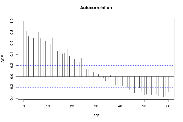
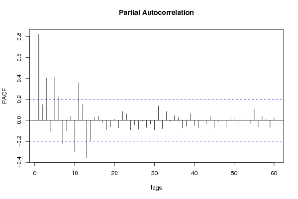
Title produced by software

(Partial) Autocorrelation Function

Date of computation

Mon, 08 Dec 2008 12:45:51 -0700

Cite this page as follows

Statistical Computations at FreeStatistics.org, Office for Research Development and Education, URL https://freestatistics.org/blog/index.php?v=date/2008/Dec/08/t1228765578wt1p2539t4wxjkf.htm/, Retrieved Thu, 16 May 2024 14:44:46 +0000

Statistical Computations at FreeStatistics.org, Office for Research Development and Education, URL https://freestatistics.org/blog/index.php?pk=30857, Retrieved Thu, 16 May 2024 14:44:46 +0000

QR Codes:

Paste this QR Code to cite your computation.

Original text written by user:

IsPrivate?

No (this computation is public)

User-defined keywords

Estimated Impact

144

Family? (F = Feedback message, R = changed R code, M = changed R Module, P = changed Parameters, D = changed Data)

-     [Univariate Data Series] [data set] [2008-12-01 19:54:57] [b98453cac15ba1066b407e146608df68]
F RMPD  [Standard Deviation-Mean Plot] [step 1] [2008-12-08 19:31:21] [5161246d1ccc1b670cc664d03050f084]
F RM D    [Variance Reduction Matrix] [step 2] [2008-12-08 19:34:58] [5161246d1ccc1b670cc664d03050f084]
F RMP       [Spectral Analysis] [step 2] [2008-12-08 19:40:15] [5161246d1ccc1b670cc664d03050f084]
- RMP           [(Partial) Autocorrelation Function] [step 2] [2008-12-08 19:45:51] [e515c0250d6233b5d2604259ab52cebe] [Current]
F   P             [(Partial) Autocorrelation Function] [step3] [2008-12-08 19:51:58] [5161246d1ccc1b670cc664d03050f084] 
F RMPD              [ARIMA Backward Selection] [] [2008-12-08 20:09:39] [5161246d1ccc1b670cc664d03050f084] 
-   PD                [ARIMA Backward Selection] [verbetering stap 5] [2008-12-15 16:48:15] [e43247bc0ab243a5af99ac7f55ba0b41] 
-   P               [(Partial) Autocorrelation Function] [Assessment verbet...] [2008-12-10 15:30:12] [46c5a5fbda57fdfa1d4ef48658f82a0c] 
-   P               [(Partial) Autocorrelation Function] [verbetering ] [2008-12-15 16:16:38] [e43247bc0ab243a5af99ac7f55ba0b41] 
- RMP             [ARIMA Backward Selection] [Assessment verbet...] [2008-12-10 15:38:14] [46c5a5fbda57fdfa1d4ef48658f82a0c] 
F RMP               [ARIMA Forecasting] [forecasting step 1] [2008-12-15 18:07:00] [5161246d1ccc1b670cc664d03050f084] 

Feedback Forum

Post a new message

Dataseries X:

Download CSV

Histogram

Boxplots

Summary of computational transaction
Raw Input	view raw input (R code)
Raw Output	view raw output of R engine
Computing time	2 seconds
R Server	'Herman Ole Andreas Wold' @ 193.190.124.10:1001

\begin{tabular}{lllllllll}
\hline
Summary of computational transaction \tabularnewline
Raw Input & view raw input (R code)  \tabularnewline
Raw Output & view raw output of R engine  \tabularnewline
Computing time & 2 seconds \tabularnewline
R Server & 'Herman Ole Andreas Wold' @ 193.190.124.10:1001 \tabularnewline
\hline
\end{tabular}
%Source: https://freestatistics.org/blog/index.php?pk=30857&T=0

[TABLE]
[ROW][C]Summary of computational transaction[/C][/ROW]
[ROW][C]Raw Input[/C][C]view raw input (R code) [/C][/ROW]
[ROW][C]Raw Output[/C][C]view raw output of R engine [/C][/ROW]
[ROW][C]Computing time[/C][C]2 seconds[/C][/ROW]
[ROW][C]R Server[/C][C]'Herman Ole Andreas Wold' @ 193.190.124.10:1001[/C][/ROW]
[/TABLE]
Source: https://freestatistics.org/blog/index.php?pk=30857&T=0

Globally Unique Identifier (entire table): ba.freestatistics.org/blog/index.php?pk=30857&T=0

As an alternative you can also use a QR Code:

The GUIDs for individual cells are displayed in the table below:

Summary of computational transaction
Raw Input	view raw input (R code)
Raw Output	view raw output of R engine
Computing time	2 seconds
R Server	'Herman Ole Andreas Wold' @ 193.190.124.10:1001

Autocorrelation Function
Time lag k	ACF(k)	T-STAT	P-value
1	0.819992	8.076	0
2	0.721678	7.1077	0
3	0.756211	7.4478	0
4	0.689979	6.7955	0
5	0.721083	7.1018	0
6	0.797965	7.859	0
7	0.68926	6.7884	0
8	0.616287	6.0697	0
9	0.644078	6.3434	0
10	0.544189	5.3596	0
11	0.588854	5.7995	0
12	0.700611	6.9002	0
13	0.560703	5.5223	0
14	0.459486	4.5254	9e-06
15	0.476428	4.6923	4e-06
16	0.411688	4.0547	5.1e-05
17	0.425231	4.188	3.1e-05
18	0.489371	4.8197	3e-06
19	0.37207	3.6645	0.000202
20	0.30518	3.0057	0.001687
21	0.312733	3.0801	0.001346
22	0.226212	2.2279	0.014098
23	0.259011	2.551	0.006153
24	0.338646	3.3353	0.000604
25	0.226509	2.2309	0.013997
26	0.128647	1.267	0.10409
27	0.132931	1.3092	0.096777
28	0.065247	0.6426	0.260996
29	0.07911	0.7791	0.218895
30	0.123147	1.2129	0.114065
31	0.036112	0.3557	0.361433
32	-0.022724	-0.2238	0.411688
33	-0.020478	-0.2017	0.420294
34	-0.084309	-0.8303	0.204191
35	-0.058994	-0.581	0.281285
36	0.019226	0.1893	0.425107
37	-0.072781	-0.7168	0.237606
38	-0.148724	-1.4648	0.07311
39	-0.142922	-1.4076	0.081221
40	-0.184046	-1.8126	0.03649
41	-0.173538	-1.7092	0.04531
42	-0.129759	-1.278	0.102153
43	-0.196203	-1.9324	0.028115
44	-0.242659	-2.3899	0.009392
45	-0.240434	-2.368	0.009934
46	-0.295433	-2.9097	0.002243
47	-0.271673	-2.6757	0.004378
48	-0.207223	-2.0409	0.021988
49	-0.267432	-2.6339	0.004913
50	-0.328399	-3.2344	0.000834
51	-0.320976	-3.1612	0.001048
52	-0.344711	-3.395	0.000498
53	-0.326791	-3.2185	0.000876
54	-0.281327	-2.7708	0.003352
55	-0.320419	-3.1558	0.001066
56	-0.344986	-3.3977	0.000493
57	-0.334385	-3.2933	0.000691
58	-0.361123	-3.5566	0.000291
59	-0.340677	-3.3553	0.000566
60	-0.274169	-2.7003	0.004088

\begin{tabular}{lllllllll}
\hline
Autocorrelation Function \tabularnewline
Time lag k & ACF(k) & T-STAT & P-value \tabularnewline
1 & 0.819992 & 8.076 & 0 \tabularnewline
2 & 0.721678 & 7.1077 & 0 \tabularnewline
3 & 0.756211 & 7.4478 & 0 \tabularnewline
4 & 0.689979 & 6.7955 & 0 \tabularnewline
5 & 0.721083 & 7.1018 & 0 \tabularnewline
6 & 0.797965 & 7.859 & 0 \tabularnewline
7 & 0.68926 & 6.7884 & 0 \tabularnewline
8 & 0.616287 & 6.0697 & 0 \tabularnewline
9 & 0.644078 & 6.3434 & 0 \tabularnewline
10 & 0.544189 & 5.3596 & 0 \tabularnewline
11 & 0.588854 & 5.7995 & 0 \tabularnewline
12 & 0.700611 & 6.9002 & 0 \tabularnewline
13 & 0.560703 & 5.5223 & 0 \tabularnewline
14 & 0.459486 & 4.5254 & 9e-06 \tabularnewline
15 & 0.476428 & 4.6923 & 4e-06 \tabularnewline
16 & 0.411688 & 4.0547 & 5.1e-05 \tabularnewline
17 & 0.425231 & 4.188 & 3.1e-05 \tabularnewline
18 & 0.489371 & 4.8197 & 3e-06 \tabularnewline
19 & 0.37207 & 3.6645 & 0.000202 \tabularnewline
20 & 0.30518 & 3.0057 & 0.001687 \tabularnewline
21 & 0.312733 & 3.0801 & 0.001346 \tabularnewline
22 & 0.226212 & 2.2279 & 0.014098 \tabularnewline
23 & 0.259011 & 2.551 & 0.006153 \tabularnewline
24 & 0.338646 & 3.3353 & 0.000604 \tabularnewline
25 & 0.226509 & 2.2309 & 0.013997 \tabularnewline
26 & 0.128647 & 1.267 & 0.10409 \tabularnewline
27 & 0.132931 & 1.3092 & 0.096777 \tabularnewline
28 & 0.065247 & 0.6426 & 0.260996 \tabularnewline
29 & 0.07911 & 0.7791 & 0.218895 \tabularnewline
30 & 0.123147 & 1.2129 & 0.114065 \tabularnewline
31 & 0.036112 & 0.3557 & 0.361433 \tabularnewline
32 & -0.022724 & -0.2238 & 0.411688 \tabularnewline
33 & -0.020478 & -0.2017 & 0.420294 \tabularnewline
34 & -0.084309 & -0.8303 & 0.204191 \tabularnewline
35 & -0.058994 & -0.581 & 0.281285 \tabularnewline
36 & 0.019226 & 0.1893 & 0.425107 \tabularnewline
37 & -0.072781 & -0.7168 & 0.237606 \tabularnewline
38 & -0.148724 & -1.4648 & 0.07311 \tabularnewline
39 & -0.142922 & -1.4076 & 0.081221 \tabularnewline
40 & -0.184046 & -1.8126 & 0.03649 \tabularnewline
41 & -0.173538 & -1.7092 & 0.04531 \tabularnewline
42 & -0.129759 & -1.278 & 0.102153 \tabularnewline
43 & -0.196203 & -1.9324 & 0.028115 \tabularnewline
44 & -0.242659 & -2.3899 & 0.009392 \tabularnewline
45 & -0.240434 & -2.368 & 0.009934 \tabularnewline
46 & -0.295433 & -2.9097 & 0.002243 \tabularnewline
47 & -0.271673 & -2.6757 & 0.004378 \tabularnewline
48 & -0.207223 & -2.0409 & 0.021988 \tabularnewline
49 & -0.267432 & -2.6339 & 0.004913 \tabularnewline
50 & -0.328399 & -3.2344 & 0.000834 \tabularnewline
51 & -0.320976 & -3.1612 & 0.001048 \tabularnewline
52 & -0.344711 & -3.395 & 0.000498 \tabularnewline
53 & -0.326791 & -3.2185 & 0.000876 \tabularnewline
54 & -0.281327 & -2.7708 & 0.003352 \tabularnewline
55 & -0.320419 & -3.1558 & 0.001066 \tabularnewline
56 & -0.344986 & -3.3977 & 0.000493 \tabularnewline
57 & -0.334385 & -3.2933 & 0.000691 \tabularnewline
58 & -0.361123 & -3.5566 & 0.000291 \tabularnewline
59 & -0.340677 & -3.3553 & 0.000566 \tabularnewline
60 & -0.274169 & -2.7003 & 0.004088 \tabularnewline
\hline
\end{tabular}
%Source: https://freestatistics.org/blog/index.php?pk=30857&T=1

[TABLE]
[ROW][C]Autocorrelation Function[/C][/ROW]
[ROW][C]Time lag k[/C][C]ACF(k)[/C][C]T-STAT[/C][C]P-value[/C][/ROW]
[ROW][C]1[/C][C]0.819992[/C][C]8.076[/C][C]0[/C][/ROW]
[ROW][C]2[/C][C]0.721678[/C][C]7.1077[/C][C]0[/C][/ROW]
[ROW][C]3[/C][C]0.756211[/C][C]7.4478[/C][C]0[/C][/ROW]
[ROW][C]4[/C][C]0.689979[/C][C]6.7955[/C][C]0[/C][/ROW]
[ROW][C]5[/C][C]0.721083[/C][C]7.1018[/C][C]0[/C][/ROW]
[ROW][C]6[/C][C]0.797965[/C][C]7.859[/C][C]0[/C][/ROW]
[ROW][C]7[/C][C]0.68926[/C][C]6.7884[/C][C]0[/C][/ROW]
[ROW][C]8[/C][C]0.616287[/C][C]6.0697[/C][C]0[/C][/ROW]
[ROW][C]9[/C][C]0.644078[/C][C]6.3434[/C][C]0[/C][/ROW]
[ROW][C]10[/C][C]0.544189[/C][C]5.3596[/C][C]0[/C][/ROW]
[ROW][C]11[/C][C]0.588854[/C][C]5.7995[/C][C]0[/C][/ROW]
[ROW][C]12[/C][C]0.700611[/C][C]6.9002[/C][C]0[/C][/ROW]
[ROW][C]13[/C][C]0.560703[/C][C]5.5223[/C][C]0[/C][/ROW]
[ROW][C]14[/C][C]0.459486[/C][C]4.5254[/C][C]9e-06[/C][/ROW]
[ROW][C]15[/C][C]0.476428[/C][C]4.6923[/C][C]4e-06[/C][/ROW]
[ROW][C]16[/C][C]0.411688[/C][C]4.0547[/C][C]5.1e-05[/C][/ROW]
[ROW][C]17[/C][C]0.425231[/C][C]4.188[/C][C]3.1e-05[/C][/ROW]
[ROW][C]18[/C][C]0.489371[/C][C]4.8197[/C][C]3e-06[/C][/ROW]
[ROW][C]19[/C][C]0.37207[/C][C]3.6645[/C][C]0.000202[/C][/ROW]
[ROW][C]20[/C][C]0.30518[/C][C]3.0057[/C][C]0.001687[/C][/ROW]
[ROW][C]21[/C][C]0.312733[/C][C]3.0801[/C][C]0.001346[/C][/ROW]
[ROW][C]22[/C][C]0.226212[/C][C]2.2279[/C][C]0.014098[/C][/ROW]
[ROW][C]23[/C][C]0.259011[/C][C]2.551[/C][C]0.006153[/C][/ROW]
[ROW][C]24[/C][C]0.338646[/C][C]3.3353[/C][C]0.000604[/C][/ROW]
[ROW][C]25[/C][C]0.226509[/C][C]2.2309[/C][C]0.013997[/C][/ROW]
[ROW][C]26[/C][C]0.128647[/C][C]1.267[/C][C]0.10409[/C][/ROW]
[ROW][C]27[/C][C]0.132931[/C][C]1.3092[/C][C]0.096777[/C][/ROW]
[ROW][C]28[/C][C]0.065247[/C][C]0.6426[/C][C]0.260996[/C][/ROW]
[ROW][C]29[/C][C]0.07911[/C][C]0.7791[/C][C]0.218895[/C][/ROW]
[ROW][C]30[/C][C]0.123147[/C][C]1.2129[/C][C]0.114065[/C][/ROW]
[ROW][C]31[/C][C]0.036112[/C][C]0.3557[/C][C]0.361433[/C][/ROW]
[ROW][C]32[/C][C]-0.022724[/C][C]-0.2238[/C][C]0.411688[/C][/ROW]
[ROW][C]33[/C][C]-0.020478[/C][C]-0.2017[/C][C]0.420294[/C][/ROW]
[ROW][C]34[/C][C]-0.084309[/C][C]-0.8303[/C][C]0.204191[/C][/ROW]
[ROW][C]35[/C][C]-0.058994[/C][C]-0.581[/C][C]0.281285[/C][/ROW]
[ROW][C]36[/C][C]0.019226[/C][C]0.1893[/C][C]0.425107[/C][/ROW]
[ROW][C]37[/C][C]-0.072781[/C][C]-0.7168[/C][C]0.237606[/C][/ROW]
[ROW][C]38[/C][C]-0.148724[/C][C]-1.4648[/C][C]0.07311[/C][/ROW]
[ROW][C]39[/C][C]-0.142922[/C][C]-1.4076[/C][C]0.081221[/C][/ROW]
[ROW][C]40[/C][C]-0.184046[/C][C]-1.8126[/C][C]0.03649[/C][/ROW]
[ROW][C]41[/C][C]-0.173538[/C][C]-1.7092[/C][C]0.04531[/C][/ROW]
[ROW][C]42[/C][C]-0.129759[/C][C]-1.278[/C][C]0.102153[/C][/ROW]
[ROW][C]43[/C][C]-0.196203[/C][C]-1.9324[/C][C]0.028115[/C][/ROW]
[ROW][C]44[/C][C]-0.242659[/C][C]-2.3899[/C][C]0.009392[/C][/ROW]
[ROW][C]45[/C][C]-0.240434[/C][C]-2.368[/C][C]0.009934[/C][/ROW]
[ROW][C]46[/C][C]-0.295433[/C][C]-2.9097[/C][C]0.002243[/C][/ROW]
[ROW][C]47[/C][C]-0.271673[/C][C]-2.6757[/C][C]0.004378[/C][/ROW]
[ROW][C]48[/C][C]-0.207223[/C][C]-2.0409[/C][C]0.021988[/C][/ROW]
[ROW][C]49[/C][C]-0.267432[/C][C]-2.6339[/C][C]0.004913[/C][/ROW]
[ROW][C]50[/C][C]-0.328399[/C][C]-3.2344[/C][C]0.000834[/C][/ROW]
[ROW][C]51[/C][C]-0.320976[/C][C]-3.1612[/C][C]0.001048[/C][/ROW]
[ROW][C]52[/C][C]-0.344711[/C][C]-3.395[/C][C]0.000498[/C][/ROW]
[ROW][C]53[/C][C]-0.326791[/C][C]-3.2185[/C][C]0.000876[/C][/ROW]
[ROW][C]54[/C][C]-0.281327[/C][C]-2.7708[/C][C]0.003352[/C][/ROW]
[ROW][C]55[/C][C]-0.320419[/C][C]-3.1558[/C][C]0.001066[/C][/ROW]
[ROW][C]56[/C][C]-0.344986[/C][C]-3.3977[/C][C]0.000493[/C][/ROW]
[ROW][C]57[/C][C]-0.334385[/C][C]-3.2933[/C][C]0.000691[/C][/ROW]
[ROW][C]58[/C][C]-0.361123[/C][C]-3.5566[/C][C]0.000291[/C][/ROW]
[ROW][C]59[/C][C]-0.340677[/C][C]-3.3553[/C][C]0.000566[/C][/ROW]
[ROW][C]60[/C][C]-0.274169[/C][C]-2.7003[/C][C]0.004088[/C][/ROW]
[/TABLE]
Source: https://freestatistics.org/blog/index.php?pk=30857&T=1

Globally Unique Identifier (entire table): ba.freestatistics.org/blog/index.php?pk=30857&T=1

As an alternative you can also use a QR Code:

The GUIDs for individual cells are displayed in the table below:

Autocorrelation Function
Time lag k	ACF(k)	T-STAT	P-value
1	0.819992	8.076	0
2	0.721678	7.1077	0
3	0.756211	7.4478	0
4	0.689979	6.7955	0
5	0.721083	7.1018	0
6	0.797965	7.859	0
7	0.68926	6.7884	0
8	0.616287	6.0697	0
9	0.644078	6.3434	0
10	0.544189	5.3596	0
11	0.588854	5.7995	0
12	0.700611	6.9002	0
13	0.560703	5.5223	0
14	0.459486	4.5254	9e-06
15	0.476428	4.6923	4e-06
16	0.411688	4.0547	5.1e-05
17	0.425231	4.188	3.1e-05
18	0.489371	4.8197	3e-06
19	0.37207	3.6645	0.000202
20	0.30518	3.0057	0.001687
21	0.312733	3.0801	0.001346
22	0.226212	2.2279	0.014098
23	0.259011	2.551	0.006153
24	0.338646	3.3353	0.000604
25	0.226509	2.2309	0.013997
26	0.128647	1.267	0.10409
27	0.132931	1.3092	0.096777
28	0.065247	0.6426	0.260996
29	0.07911	0.7791	0.218895
30	0.123147	1.2129	0.114065
31	0.036112	0.3557	0.361433
32	-0.022724	-0.2238	0.411688
33	-0.020478	-0.2017	0.420294
34	-0.084309	-0.8303	0.204191
35	-0.058994	-0.581	0.281285
36	0.019226	0.1893	0.425107
37	-0.072781	-0.7168	0.237606
38	-0.148724	-1.4648	0.07311
39	-0.142922	-1.4076	0.081221
40	-0.184046	-1.8126	0.03649
41	-0.173538	-1.7092	0.04531
42	-0.129759	-1.278	0.102153
43	-0.196203	-1.9324	0.028115
44	-0.242659	-2.3899	0.009392
45	-0.240434	-2.368	0.009934
46	-0.295433	-2.9097	0.002243
47	-0.271673	-2.6757	0.004378
48	-0.207223	-2.0409	0.021988
49	-0.267432	-2.6339	0.004913
50	-0.328399	-3.2344	0.000834
51	-0.320976	-3.1612	0.001048
52	-0.344711	-3.395	0.000498
53	-0.326791	-3.2185	0.000876
54	-0.281327	-2.7708	0.003352
55	-0.320419	-3.1558	0.001066
56	-0.344986	-3.3977	0.000493
57	-0.334385	-3.2933	0.000691
58	-0.361123	-3.5566	0.000291
59	-0.340677	-3.3553	0.000566
60	-0.274169	-2.7003	0.004088

Partial Autocorrelation Function
Time lag k	PACF(k)	T-STAT	P-value
1	0.819992	8.076	0
2	0.150456	1.4818	0.070815
3	0.406323	4.0018	6.1e-05
4	-0.105007	-1.0342	0.151808
5	0.411083	4.0487	5.2e-05
6	0.226275	2.2286	0.014076
7	-0.221096	-2.1775	0.015933
8	-0.097925	-0.9645	0.168608
9	0.038154	0.3758	0.353954
10	-0.296966	-2.9248	0.002146
11	0.361594	3.5613	0.000287
12	0.150681	1.484	0.070521
13	-0.353782	-3.4844	0.000371
14	-0.197475	-1.9449	0.027341
15	0.029231	0.2879	0.387022
16	0.04432	0.4365	0.331722
17	-0.020363	-0.2006	0.420735
18	-0.08725	-0.8593	0.196142
19	-0.06133	-0.604	0.273618
20	0.009021	0.0889	0.464692
21	-0.070293	-0.6923	0.245199
22	0.085094	0.8381	0.202023
23	0.062936	0.6198	0.268406
24	-0.093272	-0.9186	0.180286
25	-0.041806	-0.4117	0.340718
26	-0.084293	-0.8302	0.204235
27	-0.005449	-0.0537	0.478655
28	-0.066967	-0.6596	0.255552
29	-0.0333	-0.328	0.371823
30	-0.089266	-0.8792	0.190742
31	0.140087	1.3797	0.085426
32	-0.07836	-0.7718	0.221066
33	0.084309	0.8303	0.204191
34	-0.008036	-0.0791	0.468541
35	0.045399	0.4471	0.327889
36	0.026483	0.2608	0.397391
37	-0.075216	-0.7408	0.230305
38	-0.056378	-0.5553	0.289998
39	0.064816	0.6384	0.262371
40	-0.050344	-0.4958	0.310567
41	-0.069709	-0.6866	0.247001
42	-0.000286	-0.0028	0.498878
43	-0.034018	-0.335	0.369161
44	0.040947	0.4033	0.343816
45	-0.075338	-0.742	0.229943
46	-0.017477	-0.1721	0.431847
47	0.002214	0.0218	0.491325
48	-0.064942	-0.6396	0.261968
49	0.026816	0.2641	0.396128
50	0.023361	0.2301	0.409258
51	-0.02789	-0.2747	0.39207
52	-0.01138	-0.1121	0.455497
53	0.047965	0.4724	0.31885
54	-0.03079	-0.3033	0.381174
55	0.109219	1.0757	0.14237
56	-0.061622	-0.6069	0.272666
57	0.039528	0.3893	0.348953
58	0.008922	0.0879	0.465081
59	-0.06719	-0.6617	0.254853
60	0.024564	0.2419	0.404673

\begin{tabular}{lllllllll}
\hline
Partial Autocorrelation Function \tabularnewline
Time lag k & PACF(k) & T-STAT & P-value \tabularnewline
1 & 0.819992 & 8.076 & 0 \tabularnewline
2 & 0.150456 & 1.4818 & 0.070815 \tabularnewline
3 & 0.406323 & 4.0018 & 6.1e-05 \tabularnewline
4 & -0.105007 & -1.0342 & 0.151808 \tabularnewline
5 & 0.411083 & 4.0487 & 5.2e-05 \tabularnewline
6 & 0.226275 & 2.2286 & 0.014076 \tabularnewline
7 & -0.221096 & -2.1775 & 0.015933 \tabularnewline
8 & -0.097925 & -0.9645 & 0.168608 \tabularnewline
9 & 0.038154 & 0.3758 & 0.353954 \tabularnewline
10 & -0.296966 & -2.9248 & 0.002146 \tabularnewline
11 & 0.361594 & 3.5613 & 0.000287 \tabularnewline
12 & 0.150681 & 1.484 & 0.070521 \tabularnewline
13 & -0.353782 & -3.4844 & 0.000371 \tabularnewline
14 & -0.197475 & -1.9449 & 0.027341 \tabularnewline
15 & 0.029231 & 0.2879 & 0.387022 \tabularnewline
16 & 0.04432 & 0.4365 & 0.331722 \tabularnewline
17 & -0.020363 & -0.2006 & 0.420735 \tabularnewline
18 & -0.08725 & -0.8593 & 0.196142 \tabularnewline
19 & -0.06133 & -0.604 & 0.273618 \tabularnewline
20 & 0.009021 & 0.0889 & 0.464692 \tabularnewline
21 & -0.070293 & -0.6923 & 0.245199 \tabularnewline
22 & 0.085094 & 0.8381 & 0.202023 \tabularnewline
23 & 0.062936 & 0.6198 & 0.268406 \tabularnewline
24 & -0.093272 & -0.9186 & 0.180286 \tabularnewline
25 & -0.041806 & -0.4117 & 0.340718 \tabularnewline
26 & -0.084293 & -0.8302 & 0.204235 \tabularnewline
27 & -0.005449 & -0.0537 & 0.478655 \tabularnewline
28 & -0.066967 & -0.6596 & 0.255552 \tabularnewline
29 & -0.0333 & -0.328 & 0.371823 \tabularnewline
30 & -0.089266 & -0.8792 & 0.190742 \tabularnewline
31 & 0.140087 & 1.3797 & 0.085426 \tabularnewline
32 & -0.07836 & -0.7718 & 0.221066 \tabularnewline
33 & 0.084309 & 0.8303 & 0.204191 \tabularnewline
34 & -0.008036 & -0.0791 & 0.468541 \tabularnewline
35 & 0.045399 & 0.4471 & 0.327889 \tabularnewline
36 & 0.026483 & 0.2608 & 0.397391 \tabularnewline
37 & -0.075216 & -0.7408 & 0.230305 \tabularnewline
38 & -0.056378 & -0.5553 & 0.289998 \tabularnewline
39 & 0.064816 & 0.6384 & 0.262371 \tabularnewline
40 & -0.050344 & -0.4958 & 0.310567 \tabularnewline
41 & -0.069709 & -0.6866 & 0.247001 \tabularnewline
42 & -0.000286 & -0.0028 & 0.498878 \tabularnewline
43 & -0.034018 & -0.335 & 0.369161 \tabularnewline
44 & 0.040947 & 0.4033 & 0.343816 \tabularnewline
45 & -0.075338 & -0.742 & 0.229943 \tabularnewline
46 & -0.017477 & -0.1721 & 0.431847 \tabularnewline
47 & 0.002214 & 0.0218 & 0.491325 \tabularnewline
48 & -0.064942 & -0.6396 & 0.261968 \tabularnewline
49 & 0.026816 & 0.2641 & 0.396128 \tabularnewline
50 & 0.023361 & 0.2301 & 0.409258 \tabularnewline
51 & -0.02789 & -0.2747 & 0.39207 \tabularnewline
52 & -0.01138 & -0.1121 & 0.455497 \tabularnewline
53 & 0.047965 & 0.4724 & 0.31885 \tabularnewline
54 & -0.03079 & -0.3033 & 0.381174 \tabularnewline
55 & 0.109219 & 1.0757 & 0.14237 \tabularnewline
56 & -0.061622 & -0.6069 & 0.272666 \tabularnewline
57 & 0.039528 & 0.3893 & 0.348953 \tabularnewline
58 & 0.008922 & 0.0879 & 0.465081 \tabularnewline
59 & -0.06719 & -0.6617 & 0.254853 \tabularnewline
60 & 0.024564 & 0.2419 & 0.404673 \tabularnewline
\hline
\end{tabular}
%Source: https://freestatistics.org/blog/index.php?pk=30857&T=2

[TABLE]
[ROW][C]Partial Autocorrelation Function[/C][/ROW]
[ROW][C]Time lag k[/C][C]PACF(k)[/C][C]T-STAT[/C][C]P-value[/C][/ROW]
[ROW][C]1[/C][C]0.819992[/C][C]8.076[/C][C]0[/C][/ROW]
[ROW][C]2[/C][C]0.150456[/C][C]1.4818[/C][C]0.070815[/C][/ROW]
[ROW][C]3[/C][C]0.406323[/C][C]4.0018[/C][C]6.1e-05[/C][/ROW]
[ROW][C]4[/C][C]-0.105007[/C][C]-1.0342[/C][C]0.151808[/C][/ROW]
[ROW][C]5[/C][C]0.411083[/C][C]4.0487[/C][C]5.2e-05[/C][/ROW]
[ROW][C]6[/C][C]0.226275[/C][C]2.2286[/C][C]0.014076[/C][/ROW]
[ROW][C]7[/C][C]-0.221096[/C][C]-2.1775[/C][C]0.015933[/C][/ROW]
[ROW][C]8[/C][C]-0.097925[/C][C]-0.9645[/C][C]0.168608[/C][/ROW]
[ROW][C]9[/C][C]0.038154[/C][C]0.3758[/C][C]0.353954[/C][/ROW]
[ROW][C]10[/C][C]-0.296966[/C][C]-2.9248[/C][C]0.002146[/C][/ROW]
[ROW][C]11[/C][C]0.361594[/C][C]3.5613[/C][C]0.000287[/C][/ROW]
[ROW][C]12[/C][C]0.150681[/C][C]1.484[/C][C]0.070521[/C][/ROW]
[ROW][C]13[/C][C]-0.353782[/C][C]-3.4844[/C][C]0.000371[/C][/ROW]
[ROW][C]14[/C][C]-0.197475[/C][C]-1.9449[/C][C]0.027341[/C][/ROW]
[ROW][C]15[/C][C]0.029231[/C][C]0.2879[/C][C]0.387022[/C][/ROW]
[ROW][C]16[/C][C]0.04432[/C][C]0.4365[/C][C]0.331722[/C][/ROW]
[ROW][C]17[/C][C]-0.020363[/C][C]-0.2006[/C][C]0.420735[/C][/ROW]
[ROW][C]18[/C][C]-0.08725[/C][C]-0.8593[/C][C]0.196142[/C][/ROW]
[ROW][C]19[/C][C]-0.06133[/C][C]-0.604[/C][C]0.273618[/C][/ROW]
[ROW][C]20[/C][C]0.009021[/C][C]0.0889[/C][C]0.464692[/C][/ROW]
[ROW][C]21[/C][C]-0.070293[/C][C]-0.6923[/C][C]0.245199[/C][/ROW]
[ROW][C]22[/C][C]0.085094[/C][C]0.8381[/C][C]0.202023[/C][/ROW]
[ROW][C]23[/C][C]0.062936[/C][C]0.6198[/C][C]0.268406[/C][/ROW]
[ROW][C]24[/C][C]-0.093272[/C][C]-0.9186[/C][C]0.180286[/C][/ROW]
[ROW][C]25[/C][C]-0.041806[/C][C]-0.4117[/C][C]0.340718[/C][/ROW]
[ROW][C]26[/C][C]-0.084293[/C][C]-0.8302[/C][C]0.204235[/C][/ROW]
[ROW][C]27[/C][C]-0.005449[/C][C]-0.0537[/C][C]0.478655[/C][/ROW]
[ROW][C]28[/C][C]-0.066967[/C][C]-0.6596[/C][C]0.255552[/C][/ROW]
[ROW][C]29[/C][C]-0.0333[/C][C]-0.328[/C][C]0.371823[/C][/ROW]
[ROW][C]30[/C][C]-0.089266[/C][C]-0.8792[/C][C]0.190742[/C][/ROW]
[ROW][C]31[/C][C]0.140087[/C][C]1.3797[/C][C]0.085426[/C][/ROW]
[ROW][C]32[/C][C]-0.07836[/C][C]-0.7718[/C][C]0.221066[/C][/ROW]
[ROW][C]33[/C][C]0.084309[/C][C]0.8303[/C][C]0.204191[/C][/ROW]
[ROW][C]34[/C][C]-0.008036[/C][C]-0.0791[/C][C]0.468541[/C][/ROW]
[ROW][C]35[/C][C]0.045399[/C][C]0.4471[/C][C]0.327889[/C][/ROW]
[ROW][C]36[/C][C]0.026483[/C][C]0.2608[/C][C]0.397391[/C][/ROW]
[ROW][C]37[/C][C]-0.075216[/C][C]-0.7408[/C][C]0.230305[/C][/ROW]
[ROW][C]38[/C][C]-0.056378[/C][C]-0.5553[/C][C]0.289998[/C][/ROW]
[ROW][C]39[/C][C]0.064816[/C][C]0.6384[/C][C]0.262371[/C][/ROW]
[ROW][C]40[/C][C]-0.050344[/C][C]-0.4958[/C][C]0.310567[/C][/ROW]
[ROW][C]41[/C][C]-0.069709[/C][C]-0.6866[/C][C]0.247001[/C][/ROW]
[ROW][C]42[/C][C]-0.000286[/C][C]-0.0028[/C][C]0.498878[/C][/ROW]
[ROW][C]43[/C][C]-0.034018[/C][C]-0.335[/C][C]0.369161[/C][/ROW]
[ROW][C]44[/C][C]0.040947[/C][C]0.4033[/C][C]0.343816[/C][/ROW]
[ROW][C]45[/C][C]-0.075338[/C][C]-0.742[/C][C]0.229943[/C][/ROW]
[ROW][C]46[/C][C]-0.017477[/C][C]-0.1721[/C][C]0.431847[/C][/ROW]
[ROW][C]47[/C][C]0.002214[/C][C]0.0218[/C][C]0.491325[/C][/ROW]
[ROW][C]48[/C][C]-0.064942[/C][C]-0.6396[/C][C]0.261968[/C][/ROW]
[ROW][C]49[/C][C]0.026816[/C][C]0.2641[/C][C]0.396128[/C][/ROW]
[ROW][C]50[/C][C]0.023361[/C][C]0.2301[/C][C]0.409258[/C][/ROW]
[ROW][C]51[/C][C]-0.02789[/C][C]-0.2747[/C][C]0.39207[/C][/ROW]
[ROW][C]52[/C][C]-0.01138[/C][C]-0.1121[/C][C]0.455497[/C][/ROW]
[ROW][C]53[/C][C]0.047965[/C][C]0.4724[/C][C]0.31885[/C][/ROW]
[ROW][C]54[/C][C]-0.03079[/C][C]-0.3033[/C][C]0.381174[/C][/ROW]
[ROW][C]55[/C][C]0.109219[/C][C]1.0757[/C][C]0.14237[/C][/ROW]
[ROW][C]56[/C][C]-0.061622[/C][C]-0.6069[/C][C]0.272666[/C][/ROW]
[ROW][C]57[/C][C]0.039528[/C][C]0.3893[/C][C]0.348953[/C][/ROW]
[ROW][C]58[/C][C]0.008922[/C][C]0.0879[/C][C]0.465081[/C][/ROW]
[ROW][C]59[/C][C]-0.06719[/C][C]-0.6617[/C][C]0.254853[/C][/ROW]
[ROW][C]60[/C][C]0.024564[/C][C]0.2419[/C][C]0.404673[/C][/ROW]
[/TABLE]
Source: https://freestatistics.org/blog/index.php?pk=30857&T=2

Globally Unique Identifier (entire table): ba.freestatistics.org/blog/index.php?pk=30857&T=2

As an alternative you can also use a QR Code:

The GUIDs for individual cells are displayed in the table below:

Partial Autocorrelation Function
Time lag k	PACF(k)	T-STAT	P-value
1	0.819992	8.076	0
2	0.150456	1.4818	0.070815
3	0.406323	4.0018	6.1e-05
4	-0.105007	-1.0342	0.151808
5	0.411083	4.0487	5.2e-05
6	0.226275	2.2286	0.014076
7	-0.221096	-2.1775	0.015933
8	-0.097925	-0.9645	0.168608
9	0.038154	0.3758	0.353954
10	-0.296966	-2.9248	0.002146
11	0.361594	3.5613	0.000287
12	0.150681	1.484	0.070521
13	-0.353782	-3.4844	0.000371
14	-0.197475	-1.9449	0.027341
15	0.029231	0.2879	0.387022
16	0.04432	0.4365	0.331722
17	-0.020363	-0.2006	0.420735
18	-0.08725	-0.8593	0.196142
19	-0.06133	-0.604	0.273618
20	0.009021	0.0889	0.464692
21	-0.070293	-0.6923	0.245199
22	0.085094	0.8381	0.202023
23	0.062936	0.6198	0.268406
24	-0.093272	-0.9186	0.180286
25	-0.041806	-0.4117	0.340718
26	-0.084293	-0.8302	0.204235
27	-0.005449	-0.0537	0.478655
28	-0.066967	-0.6596	0.255552
29	-0.0333	-0.328	0.371823
30	-0.089266	-0.8792	0.190742
31	0.140087	1.3797	0.085426
32	-0.07836	-0.7718	0.221066
33	0.084309	0.8303	0.204191
34	-0.008036	-0.0791	0.468541
35	0.045399	0.4471	0.327889
36	0.026483	0.2608	0.397391
37	-0.075216	-0.7408	0.230305
38	-0.056378	-0.5553	0.289998
39	0.064816	0.6384	0.262371
40	-0.050344	-0.4958	0.310567
41	-0.069709	-0.6866	0.247001
42	-0.000286	-0.0028	0.498878
43	-0.034018	-0.335	0.369161
44	0.040947	0.4033	0.343816
45	-0.075338	-0.742	0.229943
46	-0.017477	-0.1721	0.431847
47	0.002214	0.0218	0.491325
48	-0.064942	-0.6396	0.261968
49	0.026816	0.2641	0.396128
50	0.023361	0.2301	0.409258
51	-0.02789	-0.2747	0.39207
52	-0.01138	-0.1121	0.455497
53	0.047965	0.4724	0.31885
54	-0.03079	-0.3033	0.381174
55	0.109219	1.0757	0.14237
56	-0.061622	-0.6069	0.272666
57	0.039528	0.3893	0.348953
58	0.008922	0.0879	0.465081
59	-0.06719	-0.6617	0.254853
60	0.024564	0.2419	0.404673

Figure 1

PNG link

Postscript link

PDF link

Figure 2

PNG link

Postscript link

PDF link

Parameters (Session):

par1 = 60 ; par2 = 1 ; par3 = 0 ; par4 = 0 ; par5 = 12 ;

Parameters (R input):

par1 = 60 ; par2 = 1 ; par3 = 0 ; par4 = 0 ; par5 = 12 ;

R code (references can be found in the software module):

if (par1 == 'Default') {
par1 = 10*log10(length(x))
} else {
par1 <- as.numeric(par1)
}
par2 <- as.numeric(par2)
par3 <- as.numeric(par3)
par4 <- as.numeric(par4)
par5 <- as.numeric(par5)
if (par2 == 0) {
x <- log(x)
} else {
x <- (x ^ par2 - 1) / par2
}
if (par3 > 0) x <- diff(x,lag=1,difference=par3)
if (par4 > 0) x <- diff(x,lag=par5,difference=par4)
bitmap(file='pic1.png')
racf <- acf(x,par1,main='Autocorrelation',xlab='lags',ylab='ACF')
dev.off()
bitmap(file='pic2.png')
rpacf <- pacf(x,par1,main='Partial Autocorrelation',xlab='lags',ylab='PACF')
dev.off()
(myacf <- c(racf$acf))
(mypacf <- c(rpacf$acf))
lengthx <- length(x)
sqrtn <- sqrt(lengthx)
load(file='createtable')
a<-table.start()
a<-table.row.start(a)
a<-table.element(a,'Autocorrelation Function',4,TRUE)
a<-table.row.end(a)
a<-table.row.start(a)
a<-table.element(a,'Time lag k',header=TRUE)
a<-table.element(a,hyperlink('basics.htm','ACF(k)','click here for more information about the Autocorrelation Function'),header=TRUE)
a<-table.element(a,'T-STAT',header=TRUE)
a<-table.element(a,'P-value',header=TRUE)
a<-table.row.end(a)
for (i in 2:(par1+1)) {
a<-table.row.start(a)
a<-table.element(a,i-1,header=TRUE)
a<-table.element(a,round(myacf[i],6))
mytstat <- myacf[i]*sqrtn
a<-table.element(a,round(mytstat,4))
a<-table.element(a,round(1-pt(abs(mytstat),lengthx),6))
a<-table.row.end(a)
}
a<-table.end(a)
table.save(a,file='mytable.tab')
a<-table.start()
a<-table.row.start(a)
a<-table.element(a,'Partial Autocorrelation Function',4,TRUE)
a<-table.row.end(a)
a<-table.row.start(a)
a<-table.element(a,'Time lag k',header=TRUE)
a<-table.element(a,hyperlink('basics.htm','PACF(k)','click here for more information about the Partial Autocorrelation Function'),header=TRUE)
a<-table.element(a,'T-STAT',header=TRUE)
a<-table.element(a,'P-value',header=TRUE)
a<-table.row.end(a)
for (i in 1:par1) {
a<-table.row.start(a)
a<-table.element(a,i,header=TRUE)
a<-table.element(a,round(mypacf[i],6))
mytstat <- mypacf[i]*sqrtn
a<-table.element(a,round(mytstat,4))
a<-table.element(a,round(1-pt(abs(mytstat),lengthx),6))
a<-table.row.end(a)
}
a<-table.end(a)
table.save(a,file='mytable1.tab')

Free Statistics

Description of Statistical Computation

Tree of Dependent Computations

Dataset

Tables (Output of Computation)

Figures (Output of Computation)

Input Parameters & R Code