Repository of Reproducible Computations

Free Statistics

of Irreproducible Research!

Author's title

Author

*The author of this computation has been verified*

R Software Module

rwasp_autocorrelation.wasp

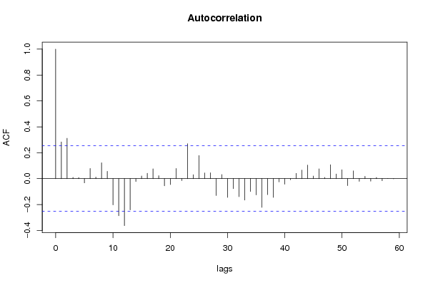
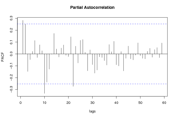
Title produced by software

(Partial) Autocorrelation Function

Date of computation

Mon, 08 Dec 2008 12:17:56 -0700

Cite this page as follows

Statistical Computations at FreeStatistics.org, Office for Research Development and Education, URL https://freestatistics.org/blog/index.php?v=date/2008/Dec/08/t1228763920fhnf09vd1wvb4sw.htm/, Retrieved Thu, 16 May 2024 10:32:25 +0000

Statistical Computations at FreeStatistics.org, Office for Research Development and Education, URL https://freestatistics.org/blog/index.php?pk=30770, Retrieved Thu, 16 May 2024 10:32:25 +0000

QR Codes:

Paste this QR Code to cite your computation.

Original text written by user:

IsPrivate?

No (this computation is public)

User-defined keywords

Estimated Impact

233

Family? (F = Feedback message, R = changed R code, M = changed R Module, P = changed Parameters, D = changed Data)

F     [Univariate Data Series] [Airline data] [2007-10-18 09:58:47] [42daae401fd3def69a25014f2252b4c2]
- RMPD  [Standard Deviation-Mean Plot] [Q5] [2008-11-29 20:10:39] [57fa5e3679c393aa19449b2f1be9928b]
-   P     [Standard Deviation-Mean Plot] [Q5] [2008-11-29 20:18:39] [57fa5e3679c393aa19449b2f1be9928b]
- RM        [Variance Reduction Matrix] [Q6 Variance] [2008-11-29 20:25:29] [57fa5e3679c393aa19449b2f1be9928b]
- RM          [(Partial) Autocorrelation Function] [Q6 ACF] [2008-11-29 20:35:57] [57fa5e3679c393aa19449b2f1be9928b]
-               [(Partial) Autocorrelation Function] [Q6 aangepaste ACF] [2008-11-29 20:44:03] [57fa5e3679c393aa19449b2f1be9928b]
- RM D            [Cross Correlation Function] [Q7] [2008-11-29 20:55:14] [57fa5e3679c393aa19449b2f1be9928b]
F RM D              [Standard Deviation-Mean Plot] [Q8 Mean plot insc...] [2008-11-29 21:03:17] [57fa5e3679c393aa19449b2f1be9928b]
F RM                  [Variance Reduction Matrix] [Q8 VRM Inschrijvi...] [2008-11-29 21:06:11] [57fa5e3679c393aa19449b2f1be9928b]
- RM                    [(Partial) Autocorrelation Function] [Q2 inschrijvingen...] [2008-12-07 14:47:46] [57fa5e3679c393aa19449b2f1be9928b]
-                         [(Partial) Autocorrelation Function] [Q3] [2008-12-07 14:59:20] [57fa5e3679c393aa19449b2f1be9928b]
-   P                         [(Partial) Autocorrelation Function] [Q3] [2008-12-08 19:17:56] [270782e2502ae87124d0ebdcd1862d6a] [Current]

Feedback Forum

Post a new message

Dataseries X:

Download CSV

Histogram

Boxplots

Summary of computational transaction
Raw Input	view raw input (R code)
Raw Output	view raw output of R engine
Computing time	3 seconds
R Server	'Sir Ronald Aylmer Fisher' @ 193.190.124.24

\begin{tabular}{lllllllll}
\hline
Summary of computational transaction \tabularnewline
Raw Input & view raw input (R code)  \tabularnewline
Raw Output & view raw output of R engine  \tabularnewline
Computing time & 3 seconds \tabularnewline
R Server & 'Sir Ronald Aylmer Fisher' @ 193.190.124.24 \tabularnewline
\hline
\end{tabular}
%Source: https://freestatistics.org/blog/index.php?pk=30770&T=0

[TABLE]
[ROW][C]Summary of computational transaction[/C][/ROW]
[ROW][C]Raw Input[/C][C]view raw input (R code) [/C][/ROW]
[ROW][C]Raw Output[/C][C]view raw output of R engine [/C][/ROW]
[ROW][C]Computing time[/C][C]3 seconds[/C][/ROW]
[ROW][C]R Server[/C][C]'Sir Ronald Aylmer Fisher' @ 193.190.124.24[/C][/ROW]
[/TABLE]
Source: https://freestatistics.org/blog/index.php?pk=30770&T=0

Globally Unique Identifier (entire table): ba.freestatistics.org/blog/index.php?pk=30770&T=0

As an alternative you can also use a QR Code:

The GUIDs for individual cells are displayed in the table below:

Summary of computational transaction
Raw Input	view raw input (R code)
Raw Output	view raw output of R engine
Computing time	3 seconds
R Server	'Sir Ronald Aylmer Fisher' @ 193.190.124.24

Autocorrelation Function
Time lag k	ACF(k)	T-STAT	P-value
1	0.283086	2.1928	0.016106
2	0.311359	2.4118	0.009476
3	0.009699	0.0751	0.470182
4	0.008331	0.0645	0.47438
5	-0.032884	-0.2547	0.399904
6	0.077814	0.6027	0.274476
7	0.011721	0.0908	0.46398
8	0.122767	0.9509	0.172723
9	0.05607	0.4343	0.33281
10	-0.202494	-1.5685	0.06101
11	-0.286449	-2.2188	0.015146
12	-0.362871	-2.8108	0.003333
13	-0.240823	-1.8654	0.033508
14	-0.022812	-0.1767	0.43017
15	0.020134	0.156	0.438294
16	0.040688	0.3152	0.376865
17	0.075161	0.5822	0.281308
18	0.022591	0.175	0.430838
19	-0.055475	-0.4297	0.334475
20	-0.045599	-0.3532	0.362586
21	0.078063	0.6047	0.273839
22	-0.015876	-0.123	0.451268
23	0.269438	2.0871	0.02057
24	0.030204	0.234	0.407907
25	0.178104	1.3796	0.086417
26	0.043531	0.3372	0.368575
27	0.045716	0.3541	0.362247
28	-0.130555	-1.0113	0.157974
29	0.031677	0.2454	0.403505
30	-0.144798	-1.1216	0.13325
31	-0.077694	-0.6018	0.274782
32	-0.139171	-1.078	0.142671
33	-0.165926	-1.2853	0.10182
34	-0.09903	-0.7671	0.223019
35	-0.125592	-0.9728	0.167272
36	-0.221891	-1.7188	0.045407
37	-0.123632	-0.9577	0.171041
38	-0.144642	-1.1204	0.133506
39	-0.025383	-0.1966	0.422395
40	-0.042846	-0.3319	0.370566
41	-0.008597	-0.0666	0.473563
42	0.040544	0.3141	0.377284
43	0.065759	0.5094	0.306181
44	0.104107	0.8064	0.211596
45	0.019886	0.154	0.439048
46	0.075632	0.5858	0.280089
47	0.0092	0.0713	0.471713
48	0.107415	0.832	0.204344
49	0.035318	0.2736	0.392678
50	0.068512	0.5307	0.298796
51	-0.053887	-0.4174	0.338935
52	0.059774	0.463	0.322517
53	-0.02158	-0.1672	0.433905
54	0.018029	0.1396	0.444702
55	-0.019803	-0.1534	0.439302
56	0.008771	0.0679	0.473031
57	-0.01634	-0.1266	0.449851
58	-0.000337	-0.0026	0.498964
59	-0.002112	-0.0164	0.493501
60	NA	NA	NA

\begin{tabular}{lllllllll}
\hline
Autocorrelation Function \tabularnewline
Time lag k & ACF(k) & T-STAT & P-value \tabularnewline
1 & 0.283086 & 2.1928 & 0.016106 \tabularnewline
2 & 0.311359 & 2.4118 & 0.009476 \tabularnewline
3 & 0.009699 & 0.0751 & 0.470182 \tabularnewline
4 & 0.008331 & 0.0645 & 0.47438 \tabularnewline
5 & -0.032884 & -0.2547 & 0.399904 \tabularnewline
6 & 0.077814 & 0.6027 & 0.274476 \tabularnewline
7 & 0.011721 & 0.0908 & 0.46398 \tabularnewline
8 & 0.122767 & 0.9509 & 0.172723 \tabularnewline
9 & 0.05607 & 0.4343 & 0.33281 \tabularnewline
10 & -0.202494 & -1.5685 & 0.06101 \tabularnewline
11 & -0.286449 & -2.2188 & 0.015146 \tabularnewline
12 & -0.362871 & -2.8108 & 0.003333 \tabularnewline
13 & -0.240823 & -1.8654 & 0.033508 \tabularnewline
14 & -0.022812 & -0.1767 & 0.43017 \tabularnewline
15 & 0.020134 & 0.156 & 0.438294 \tabularnewline
16 & 0.040688 & 0.3152 & 0.376865 \tabularnewline
17 & 0.075161 & 0.5822 & 0.281308 \tabularnewline
18 & 0.022591 & 0.175 & 0.430838 \tabularnewline
19 & -0.055475 & -0.4297 & 0.334475 \tabularnewline
20 & -0.045599 & -0.3532 & 0.362586 \tabularnewline
21 & 0.078063 & 0.6047 & 0.273839 \tabularnewline
22 & -0.015876 & -0.123 & 0.451268 \tabularnewline
23 & 0.269438 & 2.0871 & 0.02057 \tabularnewline
24 & 0.030204 & 0.234 & 0.407907 \tabularnewline
25 & 0.178104 & 1.3796 & 0.086417 \tabularnewline
26 & 0.043531 & 0.3372 & 0.368575 \tabularnewline
27 & 0.045716 & 0.3541 & 0.362247 \tabularnewline
28 & -0.130555 & -1.0113 & 0.157974 \tabularnewline
29 & 0.031677 & 0.2454 & 0.403505 \tabularnewline
30 & -0.144798 & -1.1216 & 0.13325 \tabularnewline
31 & -0.077694 & -0.6018 & 0.274782 \tabularnewline
32 & -0.139171 & -1.078 & 0.142671 \tabularnewline
33 & -0.165926 & -1.2853 & 0.10182 \tabularnewline
34 & -0.09903 & -0.7671 & 0.223019 \tabularnewline
35 & -0.125592 & -0.9728 & 0.167272 \tabularnewline
36 & -0.221891 & -1.7188 & 0.045407 \tabularnewline
37 & -0.123632 & -0.9577 & 0.171041 \tabularnewline
38 & -0.144642 & -1.1204 & 0.133506 \tabularnewline
39 & -0.025383 & -0.1966 & 0.422395 \tabularnewline
40 & -0.042846 & -0.3319 & 0.370566 \tabularnewline
41 & -0.008597 & -0.0666 & 0.473563 \tabularnewline
42 & 0.040544 & 0.3141 & 0.377284 \tabularnewline
43 & 0.065759 & 0.5094 & 0.306181 \tabularnewline
44 & 0.104107 & 0.8064 & 0.211596 \tabularnewline
45 & 0.019886 & 0.154 & 0.439048 \tabularnewline
46 & 0.075632 & 0.5858 & 0.280089 \tabularnewline
47 & 0.0092 & 0.0713 & 0.471713 \tabularnewline
48 & 0.107415 & 0.832 & 0.204344 \tabularnewline
49 & 0.035318 & 0.2736 & 0.392678 \tabularnewline
50 & 0.068512 & 0.5307 & 0.298796 \tabularnewline
51 & -0.053887 & -0.4174 & 0.338935 \tabularnewline
52 & 0.059774 & 0.463 & 0.322517 \tabularnewline
53 & -0.02158 & -0.1672 & 0.433905 \tabularnewline
54 & 0.018029 & 0.1396 & 0.444702 \tabularnewline
55 & -0.019803 & -0.1534 & 0.439302 \tabularnewline
56 & 0.008771 & 0.0679 & 0.473031 \tabularnewline
57 & -0.01634 & -0.1266 & 0.449851 \tabularnewline
58 & -0.000337 & -0.0026 & 0.498964 \tabularnewline
59 & -0.002112 & -0.0164 & 0.493501 \tabularnewline
60 & NA & NA & NA \tabularnewline
\hline
\end{tabular}
%Source: https://freestatistics.org/blog/index.php?pk=30770&T=1

[TABLE]
[ROW][C]Autocorrelation Function[/C][/ROW]
[ROW][C]Time lag k[/C][C]ACF(k)[/C][C]T-STAT[/C][C]P-value[/C][/ROW]
[ROW][C]1[/C][C]0.283086[/C][C]2.1928[/C][C]0.016106[/C][/ROW]
[ROW][C]2[/C][C]0.311359[/C][C]2.4118[/C][C]0.009476[/C][/ROW]
[ROW][C]3[/C][C]0.009699[/C][C]0.0751[/C][C]0.470182[/C][/ROW]
[ROW][C]4[/C][C]0.008331[/C][C]0.0645[/C][C]0.47438[/C][/ROW]
[ROW][C]5[/C][C]-0.032884[/C][C]-0.2547[/C][C]0.399904[/C][/ROW]
[ROW][C]6[/C][C]0.077814[/C][C]0.6027[/C][C]0.274476[/C][/ROW]
[ROW][C]7[/C][C]0.011721[/C][C]0.0908[/C][C]0.46398[/C][/ROW]
[ROW][C]8[/C][C]0.122767[/C][C]0.9509[/C][C]0.172723[/C][/ROW]
[ROW][C]9[/C][C]0.05607[/C][C]0.4343[/C][C]0.33281[/C][/ROW]
[ROW][C]10[/C][C]-0.202494[/C][C]-1.5685[/C][C]0.06101[/C][/ROW]
[ROW][C]11[/C][C]-0.286449[/C][C]-2.2188[/C][C]0.015146[/C][/ROW]
[ROW][C]12[/C][C]-0.362871[/C][C]-2.8108[/C][C]0.003333[/C][/ROW]
[ROW][C]13[/C][C]-0.240823[/C][C]-1.8654[/C][C]0.033508[/C][/ROW]
[ROW][C]14[/C][C]-0.022812[/C][C]-0.1767[/C][C]0.43017[/C][/ROW]
[ROW][C]15[/C][C]0.020134[/C][C]0.156[/C][C]0.438294[/C][/ROW]
[ROW][C]16[/C][C]0.040688[/C][C]0.3152[/C][C]0.376865[/C][/ROW]
[ROW][C]17[/C][C]0.075161[/C][C]0.5822[/C][C]0.281308[/C][/ROW]
[ROW][C]18[/C][C]0.022591[/C][C]0.175[/C][C]0.430838[/C][/ROW]
[ROW][C]19[/C][C]-0.055475[/C][C]-0.4297[/C][C]0.334475[/C][/ROW]
[ROW][C]20[/C][C]-0.045599[/C][C]-0.3532[/C][C]0.362586[/C][/ROW]
[ROW][C]21[/C][C]0.078063[/C][C]0.6047[/C][C]0.273839[/C][/ROW]
[ROW][C]22[/C][C]-0.015876[/C][C]-0.123[/C][C]0.451268[/C][/ROW]
[ROW][C]23[/C][C]0.269438[/C][C]2.0871[/C][C]0.02057[/C][/ROW]
[ROW][C]24[/C][C]0.030204[/C][C]0.234[/C][C]0.407907[/C][/ROW]
[ROW][C]25[/C][C]0.178104[/C][C]1.3796[/C][C]0.086417[/C][/ROW]
[ROW][C]26[/C][C]0.043531[/C][C]0.3372[/C][C]0.368575[/C][/ROW]
[ROW][C]27[/C][C]0.045716[/C][C]0.3541[/C][C]0.362247[/C][/ROW]
[ROW][C]28[/C][C]-0.130555[/C][C]-1.0113[/C][C]0.157974[/C][/ROW]
[ROW][C]29[/C][C]0.031677[/C][C]0.2454[/C][C]0.403505[/C][/ROW]
[ROW][C]30[/C][C]-0.144798[/C][C]-1.1216[/C][C]0.13325[/C][/ROW]
[ROW][C]31[/C][C]-0.077694[/C][C]-0.6018[/C][C]0.274782[/C][/ROW]
[ROW][C]32[/C][C]-0.139171[/C][C]-1.078[/C][C]0.142671[/C][/ROW]
[ROW][C]33[/C][C]-0.165926[/C][C]-1.2853[/C][C]0.10182[/C][/ROW]
[ROW][C]34[/C][C]-0.09903[/C][C]-0.7671[/C][C]0.223019[/C][/ROW]
[ROW][C]35[/C][C]-0.125592[/C][C]-0.9728[/C][C]0.167272[/C][/ROW]
[ROW][C]36[/C][C]-0.221891[/C][C]-1.7188[/C][C]0.045407[/C][/ROW]
[ROW][C]37[/C][C]-0.123632[/C][C]-0.9577[/C][C]0.171041[/C][/ROW]
[ROW][C]38[/C][C]-0.144642[/C][C]-1.1204[/C][C]0.133506[/C][/ROW]
[ROW][C]39[/C][C]-0.025383[/C][C]-0.1966[/C][C]0.422395[/C][/ROW]
[ROW][C]40[/C][C]-0.042846[/C][C]-0.3319[/C][C]0.370566[/C][/ROW]
[ROW][C]41[/C][C]-0.008597[/C][C]-0.0666[/C][C]0.473563[/C][/ROW]
[ROW][C]42[/C][C]0.040544[/C][C]0.3141[/C][C]0.377284[/C][/ROW]
[ROW][C]43[/C][C]0.065759[/C][C]0.5094[/C][C]0.306181[/C][/ROW]
[ROW][C]44[/C][C]0.104107[/C][C]0.8064[/C][C]0.211596[/C][/ROW]
[ROW][C]45[/C][C]0.019886[/C][C]0.154[/C][C]0.439048[/C][/ROW]
[ROW][C]46[/C][C]0.075632[/C][C]0.5858[/C][C]0.280089[/C][/ROW]
[ROW][C]47[/C][C]0.0092[/C][C]0.0713[/C][C]0.471713[/C][/ROW]
[ROW][C]48[/C][C]0.107415[/C][C]0.832[/C][C]0.204344[/C][/ROW]
[ROW][C]49[/C][C]0.035318[/C][C]0.2736[/C][C]0.392678[/C][/ROW]
[ROW][C]50[/C][C]0.068512[/C][C]0.5307[/C][C]0.298796[/C][/ROW]
[ROW][C]51[/C][C]-0.053887[/C][C]-0.4174[/C][C]0.338935[/C][/ROW]
[ROW][C]52[/C][C]0.059774[/C][C]0.463[/C][C]0.322517[/C][/ROW]
[ROW][C]53[/C][C]-0.02158[/C][C]-0.1672[/C][C]0.433905[/C][/ROW]
[ROW][C]54[/C][C]0.018029[/C][C]0.1396[/C][C]0.444702[/C][/ROW]
[ROW][C]55[/C][C]-0.019803[/C][C]-0.1534[/C][C]0.439302[/C][/ROW]
[ROW][C]56[/C][C]0.008771[/C][C]0.0679[/C][C]0.473031[/C][/ROW]
[ROW][C]57[/C][C]-0.01634[/C][C]-0.1266[/C][C]0.449851[/C][/ROW]
[ROW][C]58[/C][C]-0.000337[/C][C]-0.0026[/C][C]0.498964[/C][/ROW]
[ROW][C]59[/C][C]-0.002112[/C][C]-0.0164[/C][C]0.493501[/C][/ROW]
[ROW][C]60[/C][C]NA[/C][C]NA[/C][C]NA[/C][/ROW]
[/TABLE]
Source: https://freestatistics.org/blog/index.php?pk=30770&T=1

Globally Unique Identifier (entire table): ba.freestatistics.org/blog/index.php?pk=30770&T=1

As an alternative you can also use a QR Code:

The GUIDs for individual cells are displayed in the table below:

Autocorrelation Function
Time lag k	ACF(k)	T-STAT	P-value
1	0.283086	2.1928	0.016106
2	0.311359	2.4118	0.009476
3	0.009699	0.0751	0.470182
4	0.008331	0.0645	0.47438
5	-0.032884	-0.2547	0.399904
6	0.077814	0.6027	0.274476
7	0.011721	0.0908	0.46398
8	0.122767	0.9509	0.172723
9	0.05607	0.4343	0.33281
10	-0.202494	-1.5685	0.06101
11	-0.286449	-2.2188	0.015146
12	-0.362871	-2.8108	0.003333
13	-0.240823	-1.8654	0.033508
14	-0.022812	-0.1767	0.43017
15	0.020134	0.156	0.438294
16	0.040688	0.3152	0.376865
17	0.075161	0.5822	0.281308
18	0.022591	0.175	0.430838
19	-0.055475	-0.4297	0.334475
20	-0.045599	-0.3532	0.362586
21	0.078063	0.6047	0.273839
22	-0.015876	-0.123	0.451268
23	0.269438	2.0871	0.02057
24	0.030204	0.234	0.407907
25	0.178104	1.3796	0.086417
26	0.043531	0.3372	0.368575
27	0.045716	0.3541	0.362247
28	-0.130555	-1.0113	0.157974
29	0.031677	0.2454	0.403505
30	-0.144798	-1.1216	0.13325
31	-0.077694	-0.6018	0.274782
32	-0.139171	-1.078	0.142671
33	-0.165926	-1.2853	0.10182
34	-0.09903	-0.7671	0.223019
35	-0.125592	-0.9728	0.167272
36	-0.221891	-1.7188	0.045407
37	-0.123632	-0.9577	0.171041
38	-0.144642	-1.1204	0.133506
39	-0.025383	-0.1966	0.422395
40	-0.042846	-0.3319	0.370566
41	-0.008597	-0.0666	0.473563
42	0.040544	0.3141	0.377284
43	0.065759	0.5094	0.306181
44	0.104107	0.8064	0.211596
45	0.019886	0.154	0.439048
46	0.075632	0.5858	0.280089
47	0.0092	0.0713	0.471713
48	0.107415	0.832	0.204344
49	0.035318	0.2736	0.392678
50	0.068512	0.5307	0.298796
51	-0.053887	-0.4174	0.338935
52	0.059774	0.463	0.322517
53	-0.02158	-0.1672	0.433905
54	0.018029	0.1396	0.444702
55	-0.019803	-0.1534	0.439302
56	0.008771	0.0679	0.473031
57	-0.01634	-0.1266	0.449851
58	-0.000337	-0.0026	0.498964
59	-0.002112	-0.0164	0.493501
60	NA	NA	NA

Partial Autocorrelation Function
Time lag k	PACF(k)	T-STAT	P-value
1	0.283086	2.1928	0.016106
2	0.251365	1.9471	0.028106
3	-0.147892	-1.1456	0.128261
4	-0.047743	-0.3698	0.356412
5	0.021506	0.1666	0.434128
6	0.113128	0.8763	0.192185
7	-0.030411	-0.2356	0.407288
8	0.076917	0.5958	0.276776
9	0.026865	0.2081	0.417931
10	-0.33251	-2.5756	0.006244
11	-0.236957	-1.8355	0.035697
12	-0.128185	-0.9929	0.162369
13	-0.00198	-0.0153	0.493906
14	0.172742	1.3381	0.092964
15	0.042078	0.3259	0.372804
16	-0.026132	-0.2024	0.420139
17	0.04935	0.3823	0.351808
18	0.075858	0.5876	0.279506
19	-0.010785	-0.0835	0.466849
20	-0.022186	-0.1718	0.432067
21	0.144421	1.1187	0.133868
22	-0.272991	-2.1146	0.019315
23	0.065329	0.506	0.307343
24	-0.075904	-0.5879	0.279386
25	0.114577	0.8875	0.189175
26	0.121275	0.9394	0.175648
27	0.013388	0.1037	0.458876
28	-0.142004	-1.1	0.137872
29	0.034497	0.2672	0.395111
30	-0.089739	-0.6951	0.244832
31	-0.16165	-1.2521	0.107689
32	-0.135939	-1.053	0.148286
33	-0.024854	-0.1925	0.423994
34	-0.030465	-0.236	0.407124
35	-0.056142	-0.4349	0.332607
36	-0.093629	-0.7252	0.23556
37	0.079094	0.6127	0.271209
38	0.018638	0.1444	0.442848
39	0.1065	0.8249	0.206334
40	-0.091242	-0.7068	0.241226
41	-0.100949	-0.7819	0.218661
42	0.020359	0.1577	0.43761
43	-0.142667	-1.1051	0.136765
44	-0.03674	-0.2846	0.38847
45	0.066259	0.5132	0.304835
46	-0.041173	-0.3189	0.375447
47	-0.049812	-0.3858	0.350488
48	-0.009552	-0.074	0.470633
49	0.093355	0.7231	0.236208
50	-0.014186	-0.1099	0.456434
51	-0.037209	-0.2882	0.387086
52	-0.041241	-0.3195	0.375247
53	0.022166	0.1717	0.432128
54	0.047757	0.3699	0.356372
55	-0.027669	-0.2143	0.415509
56	0.037101	0.2874	0.387403
57	0.053611	0.4153	0.339714
58	-0.030971	-0.2399	0.405612
59	0.092222	0.7143	0.238892
60	NA	NA	NA

\begin{tabular}{lllllllll}
\hline
Partial Autocorrelation Function \tabularnewline
Time lag k & PACF(k) & T-STAT & P-value \tabularnewline
1 & 0.283086 & 2.1928 & 0.016106 \tabularnewline
2 & 0.251365 & 1.9471 & 0.028106 \tabularnewline
3 & -0.147892 & -1.1456 & 0.128261 \tabularnewline
4 & -0.047743 & -0.3698 & 0.356412 \tabularnewline
5 & 0.021506 & 0.1666 & 0.434128 \tabularnewline
6 & 0.113128 & 0.8763 & 0.192185 \tabularnewline
7 & -0.030411 & -0.2356 & 0.407288 \tabularnewline
8 & 0.076917 & 0.5958 & 0.276776 \tabularnewline
9 & 0.026865 & 0.2081 & 0.417931 \tabularnewline
10 & -0.33251 & -2.5756 & 0.006244 \tabularnewline
11 & -0.236957 & -1.8355 & 0.035697 \tabularnewline
12 & -0.128185 & -0.9929 & 0.162369 \tabularnewline
13 & -0.00198 & -0.0153 & 0.493906 \tabularnewline
14 & 0.172742 & 1.3381 & 0.092964 \tabularnewline
15 & 0.042078 & 0.3259 & 0.372804 \tabularnewline
16 & -0.026132 & -0.2024 & 0.420139 \tabularnewline
17 & 0.04935 & 0.3823 & 0.351808 \tabularnewline
18 & 0.075858 & 0.5876 & 0.279506 \tabularnewline
19 & -0.010785 & -0.0835 & 0.466849 \tabularnewline
20 & -0.022186 & -0.1718 & 0.432067 \tabularnewline
21 & 0.144421 & 1.1187 & 0.133868 \tabularnewline
22 & -0.272991 & -2.1146 & 0.019315 \tabularnewline
23 & 0.065329 & 0.506 & 0.307343 \tabularnewline
24 & -0.075904 & -0.5879 & 0.279386 \tabularnewline
25 & 0.114577 & 0.8875 & 0.189175 \tabularnewline
26 & 0.121275 & 0.9394 & 0.175648 \tabularnewline
27 & 0.013388 & 0.1037 & 0.458876 \tabularnewline
28 & -0.142004 & -1.1 & 0.137872 \tabularnewline
29 & 0.034497 & 0.2672 & 0.395111 \tabularnewline
30 & -0.089739 & -0.6951 & 0.244832 \tabularnewline
31 & -0.16165 & -1.2521 & 0.107689 \tabularnewline
32 & -0.135939 & -1.053 & 0.148286 \tabularnewline
33 & -0.024854 & -0.1925 & 0.423994 \tabularnewline
34 & -0.030465 & -0.236 & 0.407124 \tabularnewline
35 & -0.056142 & -0.4349 & 0.332607 \tabularnewline
36 & -0.093629 & -0.7252 & 0.23556 \tabularnewline
37 & 0.079094 & 0.6127 & 0.271209 \tabularnewline
38 & 0.018638 & 0.1444 & 0.442848 \tabularnewline
39 & 0.1065 & 0.8249 & 0.206334 \tabularnewline
40 & -0.091242 & -0.7068 & 0.241226 \tabularnewline
41 & -0.100949 & -0.7819 & 0.218661 \tabularnewline
42 & 0.020359 & 0.1577 & 0.43761 \tabularnewline
43 & -0.142667 & -1.1051 & 0.136765 \tabularnewline
44 & -0.03674 & -0.2846 & 0.38847 \tabularnewline
45 & 0.066259 & 0.5132 & 0.304835 \tabularnewline
46 & -0.041173 & -0.3189 & 0.375447 \tabularnewline
47 & -0.049812 & -0.3858 & 0.350488 \tabularnewline
48 & -0.009552 & -0.074 & 0.470633 \tabularnewline
49 & 0.093355 & 0.7231 & 0.236208 \tabularnewline
50 & -0.014186 & -0.1099 & 0.456434 \tabularnewline
51 & -0.037209 & -0.2882 & 0.387086 \tabularnewline
52 & -0.041241 & -0.3195 & 0.375247 \tabularnewline
53 & 0.022166 & 0.1717 & 0.432128 \tabularnewline
54 & 0.047757 & 0.3699 & 0.356372 \tabularnewline
55 & -0.027669 & -0.2143 & 0.415509 \tabularnewline
56 & 0.037101 & 0.2874 & 0.387403 \tabularnewline
57 & 0.053611 & 0.4153 & 0.339714 \tabularnewline
58 & -0.030971 & -0.2399 & 0.405612 \tabularnewline
59 & 0.092222 & 0.7143 & 0.238892 \tabularnewline
60 & NA & NA & NA \tabularnewline
\hline
\end{tabular}
%Source: https://freestatistics.org/blog/index.php?pk=30770&T=2

[TABLE]
[ROW][C]Partial Autocorrelation Function[/C][/ROW]
[ROW][C]Time lag k[/C][C]PACF(k)[/C][C]T-STAT[/C][C]P-value[/C][/ROW]
[ROW][C]1[/C][C]0.283086[/C][C]2.1928[/C][C]0.016106[/C][/ROW]
[ROW][C]2[/C][C]0.251365[/C][C]1.9471[/C][C]0.028106[/C][/ROW]
[ROW][C]3[/C][C]-0.147892[/C][C]-1.1456[/C][C]0.128261[/C][/ROW]
[ROW][C]4[/C][C]-0.047743[/C][C]-0.3698[/C][C]0.356412[/C][/ROW]
[ROW][C]5[/C][C]0.021506[/C][C]0.1666[/C][C]0.434128[/C][/ROW]
[ROW][C]6[/C][C]0.113128[/C][C]0.8763[/C][C]0.192185[/C][/ROW]
[ROW][C]7[/C][C]-0.030411[/C][C]-0.2356[/C][C]0.407288[/C][/ROW]
[ROW][C]8[/C][C]0.076917[/C][C]0.5958[/C][C]0.276776[/C][/ROW]
[ROW][C]9[/C][C]0.026865[/C][C]0.2081[/C][C]0.417931[/C][/ROW]
[ROW][C]10[/C][C]-0.33251[/C][C]-2.5756[/C][C]0.006244[/C][/ROW]
[ROW][C]11[/C][C]-0.236957[/C][C]-1.8355[/C][C]0.035697[/C][/ROW]
[ROW][C]12[/C][C]-0.128185[/C][C]-0.9929[/C][C]0.162369[/C][/ROW]
[ROW][C]13[/C][C]-0.00198[/C][C]-0.0153[/C][C]0.493906[/C][/ROW]
[ROW][C]14[/C][C]0.172742[/C][C]1.3381[/C][C]0.092964[/C][/ROW]
[ROW][C]15[/C][C]0.042078[/C][C]0.3259[/C][C]0.372804[/C][/ROW]
[ROW][C]16[/C][C]-0.026132[/C][C]-0.2024[/C][C]0.420139[/C][/ROW]
[ROW][C]17[/C][C]0.04935[/C][C]0.3823[/C][C]0.351808[/C][/ROW]
[ROW][C]18[/C][C]0.075858[/C][C]0.5876[/C][C]0.279506[/C][/ROW]
[ROW][C]19[/C][C]-0.010785[/C][C]-0.0835[/C][C]0.466849[/C][/ROW]
[ROW][C]20[/C][C]-0.022186[/C][C]-0.1718[/C][C]0.432067[/C][/ROW]
[ROW][C]21[/C][C]0.144421[/C][C]1.1187[/C][C]0.133868[/C][/ROW]
[ROW][C]22[/C][C]-0.272991[/C][C]-2.1146[/C][C]0.019315[/C][/ROW]
[ROW][C]23[/C][C]0.065329[/C][C]0.506[/C][C]0.307343[/C][/ROW]
[ROW][C]24[/C][C]-0.075904[/C][C]-0.5879[/C][C]0.279386[/C][/ROW]
[ROW][C]25[/C][C]0.114577[/C][C]0.8875[/C][C]0.189175[/C][/ROW]
[ROW][C]26[/C][C]0.121275[/C][C]0.9394[/C][C]0.175648[/C][/ROW]
[ROW][C]27[/C][C]0.013388[/C][C]0.1037[/C][C]0.458876[/C][/ROW]
[ROW][C]28[/C][C]-0.142004[/C][C]-1.1[/C][C]0.137872[/C][/ROW]
[ROW][C]29[/C][C]0.034497[/C][C]0.2672[/C][C]0.395111[/C][/ROW]
[ROW][C]30[/C][C]-0.089739[/C][C]-0.6951[/C][C]0.244832[/C][/ROW]
[ROW][C]31[/C][C]-0.16165[/C][C]-1.2521[/C][C]0.107689[/C][/ROW]
[ROW][C]32[/C][C]-0.135939[/C][C]-1.053[/C][C]0.148286[/C][/ROW]
[ROW][C]33[/C][C]-0.024854[/C][C]-0.1925[/C][C]0.423994[/C][/ROW]
[ROW][C]34[/C][C]-0.030465[/C][C]-0.236[/C][C]0.407124[/C][/ROW]
[ROW][C]35[/C][C]-0.056142[/C][C]-0.4349[/C][C]0.332607[/C][/ROW]
[ROW][C]36[/C][C]-0.093629[/C][C]-0.7252[/C][C]0.23556[/C][/ROW]
[ROW][C]37[/C][C]0.079094[/C][C]0.6127[/C][C]0.271209[/C][/ROW]
[ROW][C]38[/C][C]0.018638[/C][C]0.1444[/C][C]0.442848[/C][/ROW]
[ROW][C]39[/C][C]0.1065[/C][C]0.8249[/C][C]0.206334[/C][/ROW]
[ROW][C]40[/C][C]-0.091242[/C][C]-0.7068[/C][C]0.241226[/C][/ROW]
[ROW][C]41[/C][C]-0.100949[/C][C]-0.7819[/C][C]0.218661[/C][/ROW]
[ROW][C]42[/C][C]0.020359[/C][C]0.1577[/C][C]0.43761[/C][/ROW]
[ROW][C]43[/C][C]-0.142667[/C][C]-1.1051[/C][C]0.136765[/C][/ROW]
[ROW][C]44[/C][C]-0.03674[/C][C]-0.2846[/C][C]0.38847[/C][/ROW]
[ROW][C]45[/C][C]0.066259[/C][C]0.5132[/C][C]0.304835[/C][/ROW]
[ROW][C]46[/C][C]-0.041173[/C][C]-0.3189[/C][C]0.375447[/C][/ROW]
[ROW][C]47[/C][C]-0.049812[/C][C]-0.3858[/C][C]0.350488[/C][/ROW]
[ROW][C]48[/C][C]-0.009552[/C][C]-0.074[/C][C]0.470633[/C][/ROW]
[ROW][C]49[/C][C]0.093355[/C][C]0.7231[/C][C]0.236208[/C][/ROW]
[ROW][C]50[/C][C]-0.014186[/C][C]-0.1099[/C][C]0.456434[/C][/ROW]
[ROW][C]51[/C][C]-0.037209[/C][C]-0.2882[/C][C]0.387086[/C][/ROW]
[ROW][C]52[/C][C]-0.041241[/C][C]-0.3195[/C][C]0.375247[/C][/ROW]
[ROW][C]53[/C][C]0.022166[/C][C]0.1717[/C][C]0.432128[/C][/ROW]
[ROW][C]54[/C][C]0.047757[/C][C]0.3699[/C][C]0.356372[/C][/ROW]
[ROW][C]55[/C][C]-0.027669[/C][C]-0.2143[/C][C]0.415509[/C][/ROW]
[ROW][C]56[/C][C]0.037101[/C][C]0.2874[/C][C]0.387403[/C][/ROW]
[ROW][C]57[/C][C]0.053611[/C][C]0.4153[/C][C]0.339714[/C][/ROW]
[ROW][C]58[/C][C]-0.030971[/C][C]-0.2399[/C][C]0.405612[/C][/ROW]
[ROW][C]59[/C][C]0.092222[/C][C]0.7143[/C][C]0.238892[/C][/ROW]
[ROW][C]60[/C][C]NA[/C][C]NA[/C][C]NA[/C][/ROW]
[/TABLE]
Source: https://freestatistics.org/blog/index.php?pk=30770&T=2

Globally Unique Identifier (entire table): ba.freestatistics.org/blog/index.php?pk=30770&T=2

As an alternative you can also use a QR Code:

The GUIDs for individual cells are displayed in the table below:

Partial Autocorrelation Function
Time lag k	PACF(k)	T-STAT	P-value
1	0.283086	2.1928	0.016106
2	0.251365	1.9471	0.028106
3	-0.147892	-1.1456	0.128261
4	-0.047743	-0.3698	0.356412
5	0.021506	0.1666	0.434128
6	0.113128	0.8763	0.192185
7	-0.030411	-0.2356	0.407288
8	0.076917	0.5958	0.276776
9	0.026865	0.2081	0.417931
10	-0.33251	-2.5756	0.006244
11	-0.236957	-1.8355	0.035697
12	-0.128185	-0.9929	0.162369
13	-0.00198	-0.0153	0.493906
14	0.172742	1.3381	0.092964
15	0.042078	0.3259	0.372804
16	-0.026132	-0.2024	0.420139
17	0.04935	0.3823	0.351808
18	0.075858	0.5876	0.279506
19	-0.010785	-0.0835	0.466849
20	-0.022186	-0.1718	0.432067
21	0.144421	1.1187	0.133868
22	-0.272991	-2.1146	0.019315
23	0.065329	0.506	0.307343
24	-0.075904	-0.5879	0.279386
25	0.114577	0.8875	0.189175
26	0.121275	0.9394	0.175648
27	0.013388	0.1037	0.458876
28	-0.142004	-1.1	0.137872
29	0.034497	0.2672	0.395111
30	-0.089739	-0.6951	0.244832
31	-0.16165	-1.2521	0.107689
32	-0.135939	-1.053	0.148286
33	-0.024854	-0.1925	0.423994
34	-0.030465	-0.236	0.407124
35	-0.056142	-0.4349	0.332607
36	-0.093629	-0.7252	0.23556
37	0.079094	0.6127	0.271209
38	0.018638	0.1444	0.442848
39	0.1065	0.8249	0.206334
40	-0.091242	-0.7068	0.241226
41	-0.100949	-0.7819	0.218661
42	0.020359	0.1577	0.43761
43	-0.142667	-1.1051	0.136765
44	-0.03674	-0.2846	0.38847
45	0.066259	0.5132	0.304835
46	-0.041173	-0.3189	0.375447
47	-0.049812	-0.3858	0.350488
48	-0.009552	-0.074	0.470633
49	0.093355	0.7231	0.236208
50	-0.014186	-0.1099	0.456434
51	-0.037209	-0.2882	0.387086
52	-0.041241	-0.3195	0.375247
53	0.022166	0.1717	0.432128
54	0.047757	0.3699	0.356372
55	-0.027669	-0.2143	0.415509
56	0.037101	0.2874	0.387403
57	0.053611	0.4153	0.339714
58	-0.030971	-0.2399	0.405612
59	0.092222	0.7143	0.238892
60	NA	NA	NA

Figure 1

PNG link

Postscript link

PDF link

Figure 2

PNG link

Postscript link

PDF link

Parameters (Session):

par1 = 60 ; par2 = 0.4 ; par3 = 0 ; par4 = 1 ; par5 = 12 ;

Parameters (R input):

par1 = 60 ; par2 = 0.4 ; par3 = 0 ; par4 = 1 ; par5 = 12 ;

R code (references can be found in the software module):

if (par1 == 'Default') {
par1 = 10*log10(length(x))
} else {
par1 <- as.numeric(par1)
}
par2 <- as.numeric(par2)
par3 <- as.numeric(par3)
par4 <- as.numeric(par4)
par5 <- as.numeric(par5)
if (par2 == 0) {
x <- log(x)
} else {
x <- (x ^ par2 - 1) / par2
}
if (par3 > 0) x <- diff(x,lag=1,difference=par3)
if (par4 > 0) x <- diff(x,lag=par5,difference=par4)
bitmap(file='pic1.png')
racf <- acf(x,par1,main='Autocorrelation',xlab='lags',ylab='ACF')
dev.off()
bitmap(file='pic2.png')
rpacf <- pacf(x,par1,main='Partial Autocorrelation',xlab='lags',ylab='PACF')
dev.off()
(myacf <- c(racf$acf))
(mypacf <- c(rpacf$acf))
lengthx <- length(x)
sqrtn <- sqrt(lengthx)
load(file='createtable')
a<-table.start()
a<-table.row.start(a)
a<-table.element(a,'Autocorrelation Function',4,TRUE)
a<-table.row.end(a)
a<-table.row.start(a)
a<-table.element(a,'Time lag k',header=TRUE)
a<-table.element(a,hyperlink('basics.htm','ACF(k)','click here for more information about the Autocorrelation Function'),header=TRUE)
a<-table.element(a,'T-STAT',header=TRUE)
a<-table.element(a,'P-value',header=TRUE)
a<-table.row.end(a)
for (i in 2:(par1+1)) {
a<-table.row.start(a)
a<-table.element(a,i-1,header=TRUE)
a<-table.element(a,round(myacf[i],6))
mytstat <- myacf[i]*sqrtn
a<-table.element(a,round(mytstat,4))
a<-table.element(a,round(1-pt(abs(mytstat),lengthx),6))
a<-table.row.end(a)
}
a<-table.end(a)
table.save(a,file='mytable.tab')
a<-table.start()
a<-table.row.start(a)
a<-table.element(a,'Partial Autocorrelation Function',4,TRUE)
a<-table.row.end(a)
a<-table.row.start(a)
a<-table.element(a,'Time lag k',header=TRUE)
a<-table.element(a,hyperlink('basics.htm','PACF(k)','click here for more information about the Partial Autocorrelation Function'),header=TRUE)
a<-table.element(a,'T-STAT',header=TRUE)
a<-table.element(a,'P-value',header=TRUE)
a<-table.row.end(a)
for (i in 1:par1) {
a<-table.row.start(a)
a<-table.element(a,i,header=TRUE)
a<-table.element(a,round(mypacf[i],6))
mytstat <- mypacf[i]*sqrtn
a<-table.element(a,round(mytstat,4))
a<-table.element(a,round(1-pt(abs(mytstat),lengthx),6))
a<-table.row.end(a)
}
a<-table.end(a)
table.save(a,file='mytable1.tab')

Free Statistics

Description of Statistical Computation

Tree of Dependent Computations

Dataset

Tables (Output of Computation)

Figures (Output of Computation)

Input Parameters & R Code