Repository of Reproducible Computations

Free Statistics

of Irreproducible Research!

Author's title

Author

*The author of this computation has been verified*

R Software Module

rwasp_autocorrelation.wasp

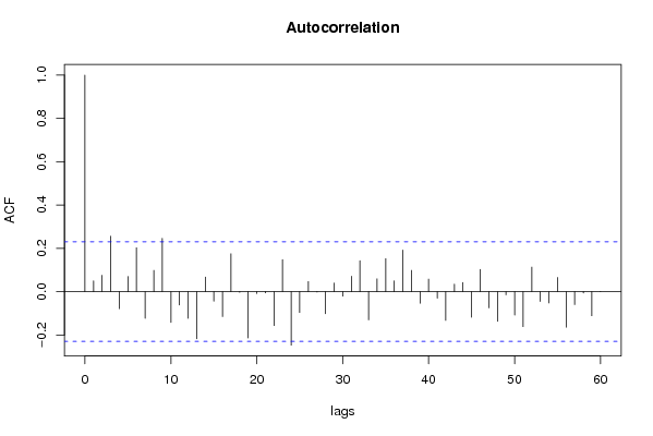
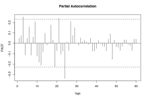
Title produced by software

(Partial) Autocorrelation Function

Date of computation

Mon, 08 Dec 2008 12:02:36 -0700

Cite this page as follows

Statistical Computations at FreeStatistics.org, Office for Research Development and Education, URL https://freestatistics.org/blog/index.php?v=date/2008/Dec/08/t1228762987s6bl3w1ghm9x75e.htm/, Retrieved Thu, 16 May 2024 06:20:12 +0000

Statistical Computations at FreeStatistics.org, Office for Research Development and Education, URL https://freestatistics.org/blog/index.php?pk=30730, Retrieved Thu, 16 May 2024 06:20:12 +0000

QR Codes:

Paste this QR Code to cite your computation.

Original text written by user:

IsPrivate?

No (this computation is public)

User-defined keywords

Estimated Impact

198

Family? (F = Feedback message, R = changed R code, M = changed R Module, P = changed Parameters, D = changed Data)

-     [Univariate Data Series] [data set] [2008-12-01 19:54:57] [b98453cac15ba1066b407e146608df68]
F RMP   [Variance Reduction Matrix] [step1.1] [2008-12-08 18:32:25] [922d8ae7bd2fd460a62d9020ccd4931a]
F RMP     [(Partial) Autocorrelation Function] [step2] [2008-12-08 18:51:58] [922d8ae7bd2fd460a62d9020ccd4931a]
F    D      [(Partial) Autocorrelation Function] [step22�] [2008-12-08 18:59:41] [922d8ae7bd2fd460a62d9020ccd4931a]
-   PD          [(Partial) Autocorrelation Function] [step223] [2008-12-08 19:02:36] [89a49ebb3ece8e9a225c7f9f53a14c57] [Current]
F RMP             [Spectral Analysis] [step45] [2008-12-08 19:13:18] [922d8ae7bd2fd460a62d9020ccd4931a] 
-   P               [Spectral Analysis] [step221] [2008-12-08 19:14:54] [922d8ae7bd2fd460a62d9020ccd4931a] 

Feedback Forum

Post a new message

Dataseries X:

Download CSV

Histogram

Boxplots

Summary of computational transaction
Raw Input	view raw input (R code)
Raw Output	view raw output of R engine
Computing time	1 seconds
R Server	'Gwilym Jenkins' @ 72.249.127.135

\begin{tabular}{lllllllll}
\hline
Summary of computational transaction \tabularnewline
Raw Input & view raw input (R code)  \tabularnewline
Raw Output & view raw output of R engine  \tabularnewline
Computing time & 1 seconds \tabularnewline
R Server & 'Gwilym Jenkins' @ 72.249.127.135 \tabularnewline
\hline
\end{tabular}
%Source: https://freestatistics.org/blog/index.php?pk=30730&T=0

[TABLE]
[ROW][C]Summary of computational transaction[/C][/ROW]
[ROW][C]Raw Input[/C][C]view raw input (R code) [/C][/ROW]
[ROW][C]Raw Output[/C][C]view raw output of R engine [/C][/ROW]
[ROW][C]Computing time[/C][C]1 seconds[/C][/ROW]
[ROW][C]R Server[/C][C]'Gwilym Jenkins' @ 72.249.127.135[/C][/ROW]
[/TABLE]
Source: https://freestatistics.org/blog/index.php?pk=30730&T=0

Globally Unique Identifier (entire table): ba.freestatistics.org/blog/index.php?pk=30730&T=0

As an alternative you can also use a QR Code:

The GUIDs for individual cells are displayed in the table below:

Summary of computational transaction
Raw Input	view raw input (R code)
Raw Output	view raw output of R engine
Computing time	1 seconds
R Server	'Gwilym Jenkins' @ 72.249.127.135

Autocorrelation Function
Time lag k	ACF(k)	T-STAT	P-value
1	0.049447	0.4225	0.33696
2	0.075338	0.6437	0.260898
3	0.255944	2.1868	0.015982
4	-0.079086	-0.6757	0.250679
5	0.069557	0.5943	0.277076
6	0.202407	1.7294	0.043985
7	-0.123561	-1.0557	0.147292
8	0.098289	0.8398	0.201887
9	0.245897	2.1009	0.01955
10	-0.142219	-1.2151	0.114117
11	-0.061772	-0.5278	0.299626
12	-0.123248	-1.053	0.1479
13	-0.217966	-1.8623	0.033292
14	0.067523	0.5769	0.282885
15	-0.044216	-0.3778	0.353344
16	-0.115137	-0.9837	0.164249
17	0.174872	1.4941	0.069729
18	-0.003031	-0.0259	0.489706
19	-0.213824	-1.8269	0.0359
20	-0.008931	-0.0763	0.469693
21	-0.005941	-0.0508	0.479829
22	-0.156868	-1.3403	0.092155
23	0.147919	1.2638	0.105158
24	-0.247278	-2.1127	0.019021
25	-0.096518	-0.8247	0.206128
26	0.046657	0.3986	0.345662
27	-0.001879	-0.0161	0.493619
28	-0.102246	-0.8736	0.192603
29	0.039662	0.3389	0.367838
30	-0.021062	-0.18	0.428844
31	0.070744	0.6044	0.273714
32	0.142729	1.2195	0.113295
33	-0.130517	-1.1151	0.134225
34	0.059094	0.5049	0.307574
35	0.15231	1.3013	0.098617
36	0.049651	0.4242	0.336327
37	0.191912	1.6397	0.052685
38	0.097922	0.8366	0.202761
39	-0.053597	-0.4579	0.32418
40	0.058039	0.4959	0.310732
41	-0.030447	-0.2601	0.397744
42	-0.132819	-1.1348	0.130085
43	0.034252	0.2926	0.38531
44	0.042038	0.3592	0.360252
45	-0.118225	-1.0101	0.157888
46	0.102432	0.8752	0.192173
47	-0.07525	-0.6429	0.261139
48	-0.137266	-1.1728	0.122345
49	-0.014765	-0.1262	0.449978
50	-0.108175	-0.9242	0.179201
51	-0.161833	-1.3827	0.085486
52	0.113433	0.9692	0.16783
53	-0.045164	-0.3859	0.350353
54	-0.052123	-0.4453	0.328697
55	0.065268	0.5577	0.289394
56	-0.164596	-1.4063	0.081938
57	-0.060191	-0.5143	0.304309
58	-0.006134	-0.0524	0.479173
59	-0.111205	-0.9501	0.17259
60	0.000568	0.0049	0.498069

\begin{tabular}{lllllllll}
\hline
Autocorrelation Function \tabularnewline
Time lag k & ACF(k) & T-STAT & P-value \tabularnewline
1 & 0.049447 & 0.4225 & 0.33696 \tabularnewline
2 & 0.075338 & 0.6437 & 0.260898 \tabularnewline
3 & 0.255944 & 2.1868 & 0.015982 \tabularnewline
4 & -0.079086 & -0.6757 & 0.250679 \tabularnewline
5 & 0.069557 & 0.5943 & 0.277076 \tabularnewline
6 & 0.202407 & 1.7294 & 0.043985 \tabularnewline
7 & -0.123561 & -1.0557 & 0.147292 \tabularnewline
8 & 0.098289 & 0.8398 & 0.201887 \tabularnewline
9 & 0.245897 & 2.1009 & 0.01955 \tabularnewline
10 & -0.142219 & -1.2151 & 0.114117 \tabularnewline
11 & -0.061772 & -0.5278 & 0.299626 \tabularnewline
12 & -0.123248 & -1.053 & 0.1479 \tabularnewline
13 & -0.217966 & -1.8623 & 0.033292 \tabularnewline
14 & 0.067523 & 0.5769 & 0.282885 \tabularnewline
15 & -0.044216 & -0.3778 & 0.353344 \tabularnewline
16 & -0.115137 & -0.9837 & 0.164249 \tabularnewline
17 & 0.174872 & 1.4941 & 0.069729 \tabularnewline
18 & -0.003031 & -0.0259 & 0.489706 \tabularnewline
19 & -0.213824 & -1.8269 & 0.0359 \tabularnewline
20 & -0.008931 & -0.0763 & 0.469693 \tabularnewline
21 & -0.005941 & -0.0508 & 0.479829 \tabularnewline
22 & -0.156868 & -1.3403 & 0.092155 \tabularnewline
23 & 0.147919 & 1.2638 & 0.105158 \tabularnewline
24 & -0.247278 & -2.1127 & 0.019021 \tabularnewline
25 & -0.096518 & -0.8247 & 0.206128 \tabularnewline
26 & 0.046657 & 0.3986 & 0.345662 \tabularnewline
27 & -0.001879 & -0.0161 & 0.493619 \tabularnewline
28 & -0.102246 & -0.8736 & 0.192603 \tabularnewline
29 & 0.039662 & 0.3389 & 0.367838 \tabularnewline
30 & -0.021062 & -0.18 & 0.428844 \tabularnewline
31 & 0.070744 & 0.6044 & 0.273714 \tabularnewline
32 & 0.142729 & 1.2195 & 0.113295 \tabularnewline
33 & -0.130517 & -1.1151 & 0.134225 \tabularnewline
34 & 0.059094 & 0.5049 & 0.307574 \tabularnewline
35 & 0.15231 & 1.3013 & 0.098617 \tabularnewline
36 & 0.049651 & 0.4242 & 0.336327 \tabularnewline
37 & 0.191912 & 1.6397 & 0.052685 \tabularnewline
38 & 0.097922 & 0.8366 & 0.202761 \tabularnewline
39 & -0.053597 & -0.4579 & 0.32418 \tabularnewline
40 & 0.058039 & 0.4959 & 0.310732 \tabularnewline
41 & -0.030447 & -0.2601 & 0.397744 \tabularnewline
42 & -0.132819 & -1.1348 & 0.130085 \tabularnewline
43 & 0.034252 & 0.2926 & 0.38531 \tabularnewline
44 & 0.042038 & 0.3592 & 0.360252 \tabularnewline
45 & -0.118225 & -1.0101 & 0.157888 \tabularnewline
46 & 0.102432 & 0.8752 & 0.192173 \tabularnewline
47 & -0.07525 & -0.6429 & 0.261139 \tabularnewline
48 & -0.137266 & -1.1728 & 0.122345 \tabularnewline
49 & -0.014765 & -0.1262 & 0.449978 \tabularnewline
50 & -0.108175 & -0.9242 & 0.179201 \tabularnewline
51 & -0.161833 & -1.3827 & 0.085486 \tabularnewline
52 & 0.113433 & 0.9692 & 0.16783 \tabularnewline
53 & -0.045164 & -0.3859 & 0.350353 \tabularnewline
54 & -0.052123 & -0.4453 & 0.328697 \tabularnewline
55 & 0.065268 & 0.5577 & 0.289394 \tabularnewline
56 & -0.164596 & -1.4063 & 0.081938 \tabularnewline
57 & -0.060191 & -0.5143 & 0.304309 \tabularnewline
58 & -0.006134 & -0.0524 & 0.479173 \tabularnewline
59 & -0.111205 & -0.9501 & 0.17259 \tabularnewline
60 & 0.000568 & 0.0049 & 0.498069 \tabularnewline
\hline
\end{tabular}
%Source: https://freestatistics.org/blog/index.php?pk=30730&T=1

[TABLE]
[ROW][C]Autocorrelation Function[/C][/ROW]
[ROW][C]Time lag k[/C][C]ACF(k)[/C][C]T-STAT[/C][C]P-value[/C][/ROW]
[ROW][C]1[/C][C]0.049447[/C][C]0.4225[/C][C]0.33696[/C][/ROW]
[ROW][C]2[/C][C]0.075338[/C][C]0.6437[/C][C]0.260898[/C][/ROW]
[ROW][C]3[/C][C]0.255944[/C][C]2.1868[/C][C]0.015982[/C][/ROW]
[ROW][C]4[/C][C]-0.079086[/C][C]-0.6757[/C][C]0.250679[/C][/ROW]
[ROW][C]5[/C][C]0.069557[/C][C]0.5943[/C][C]0.277076[/C][/ROW]
[ROW][C]6[/C][C]0.202407[/C][C]1.7294[/C][C]0.043985[/C][/ROW]
[ROW][C]7[/C][C]-0.123561[/C][C]-1.0557[/C][C]0.147292[/C][/ROW]
[ROW][C]8[/C][C]0.098289[/C][C]0.8398[/C][C]0.201887[/C][/ROW]
[ROW][C]9[/C][C]0.245897[/C][C]2.1009[/C][C]0.01955[/C][/ROW]
[ROW][C]10[/C][C]-0.142219[/C][C]-1.2151[/C][C]0.114117[/C][/ROW]
[ROW][C]11[/C][C]-0.061772[/C][C]-0.5278[/C][C]0.299626[/C][/ROW]
[ROW][C]12[/C][C]-0.123248[/C][C]-1.053[/C][C]0.1479[/C][/ROW]
[ROW][C]13[/C][C]-0.217966[/C][C]-1.8623[/C][C]0.033292[/C][/ROW]
[ROW][C]14[/C][C]0.067523[/C][C]0.5769[/C][C]0.282885[/C][/ROW]
[ROW][C]15[/C][C]-0.044216[/C][C]-0.3778[/C][C]0.353344[/C][/ROW]
[ROW][C]16[/C][C]-0.115137[/C][C]-0.9837[/C][C]0.164249[/C][/ROW]
[ROW][C]17[/C][C]0.174872[/C][C]1.4941[/C][C]0.069729[/C][/ROW]
[ROW][C]18[/C][C]-0.003031[/C][C]-0.0259[/C][C]0.489706[/C][/ROW]
[ROW][C]19[/C][C]-0.213824[/C][C]-1.8269[/C][C]0.0359[/C][/ROW]
[ROW][C]20[/C][C]-0.008931[/C][C]-0.0763[/C][C]0.469693[/C][/ROW]
[ROW][C]21[/C][C]-0.005941[/C][C]-0.0508[/C][C]0.479829[/C][/ROW]
[ROW][C]22[/C][C]-0.156868[/C][C]-1.3403[/C][C]0.092155[/C][/ROW]
[ROW][C]23[/C][C]0.147919[/C][C]1.2638[/C][C]0.105158[/C][/ROW]
[ROW][C]24[/C][C]-0.247278[/C][C]-2.1127[/C][C]0.019021[/C][/ROW]
[ROW][C]25[/C][C]-0.096518[/C][C]-0.8247[/C][C]0.206128[/C][/ROW]
[ROW][C]26[/C][C]0.046657[/C][C]0.3986[/C][C]0.345662[/C][/ROW]
[ROW][C]27[/C][C]-0.001879[/C][C]-0.0161[/C][C]0.493619[/C][/ROW]
[ROW][C]28[/C][C]-0.102246[/C][C]-0.8736[/C][C]0.192603[/C][/ROW]
[ROW][C]29[/C][C]0.039662[/C][C]0.3389[/C][C]0.367838[/C][/ROW]
[ROW][C]30[/C][C]-0.021062[/C][C]-0.18[/C][C]0.428844[/C][/ROW]
[ROW][C]31[/C][C]0.070744[/C][C]0.6044[/C][C]0.273714[/C][/ROW]
[ROW][C]32[/C][C]0.142729[/C][C]1.2195[/C][C]0.113295[/C][/ROW]
[ROW][C]33[/C][C]-0.130517[/C][C]-1.1151[/C][C]0.134225[/C][/ROW]
[ROW][C]34[/C][C]0.059094[/C][C]0.5049[/C][C]0.307574[/C][/ROW]
[ROW][C]35[/C][C]0.15231[/C][C]1.3013[/C][C]0.098617[/C][/ROW]
[ROW][C]36[/C][C]0.049651[/C][C]0.4242[/C][C]0.336327[/C][/ROW]
[ROW][C]37[/C][C]0.191912[/C][C]1.6397[/C][C]0.052685[/C][/ROW]
[ROW][C]38[/C][C]0.097922[/C][C]0.8366[/C][C]0.202761[/C][/ROW]
[ROW][C]39[/C][C]-0.053597[/C][C]-0.4579[/C][C]0.32418[/C][/ROW]
[ROW][C]40[/C][C]0.058039[/C][C]0.4959[/C][C]0.310732[/C][/ROW]
[ROW][C]41[/C][C]-0.030447[/C][C]-0.2601[/C][C]0.397744[/C][/ROW]
[ROW][C]42[/C][C]-0.132819[/C][C]-1.1348[/C][C]0.130085[/C][/ROW]
[ROW][C]43[/C][C]0.034252[/C][C]0.2926[/C][C]0.38531[/C][/ROW]
[ROW][C]44[/C][C]0.042038[/C][C]0.3592[/C][C]0.360252[/C][/ROW]
[ROW][C]45[/C][C]-0.118225[/C][C]-1.0101[/C][C]0.157888[/C][/ROW]
[ROW][C]46[/C][C]0.102432[/C][C]0.8752[/C][C]0.192173[/C][/ROW]
[ROW][C]47[/C][C]-0.07525[/C][C]-0.6429[/C][C]0.261139[/C][/ROW]
[ROW][C]48[/C][C]-0.137266[/C][C]-1.1728[/C][C]0.122345[/C][/ROW]
[ROW][C]49[/C][C]-0.014765[/C][C]-0.1262[/C][C]0.449978[/C][/ROW]
[ROW][C]50[/C][C]-0.108175[/C][C]-0.9242[/C][C]0.179201[/C][/ROW]
[ROW][C]51[/C][C]-0.161833[/C][C]-1.3827[/C][C]0.085486[/C][/ROW]
[ROW][C]52[/C][C]0.113433[/C][C]0.9692[/C][C]0.16783[/C][/ROW]
[ROW][C]53[/C][C]-0.045164[/C][C]-0.3859[/C][C]0.350353[/C][/ROW]
[ROW][C]54[/C][C]-0.052123[/C][C]-0.4453[/C][C]0.328697[/C][/ROW]
[ROW][C]55[/C][C]0.065268[/C][C]0.5577[/C][C]0.289394[/C][/ROW]
[ROW][C]56[/C][C]-0.164596[/C][C]-1.4063[/C][C]0.081938[/C][/ROW]
[ROW][C]57[/C][C]-0.060191[/C][C]-0.5143[/C][C]0.304309[/C][/ROW]
[ROW][C]58[/C][C]-0.006134[/C][C]-0.0524[/C][C]0.479173[/C][/ROW]
[ROW][C]59[/C][C]-0.111205[/C][C]-0.9501[/C][C]0.17259[/C][/ROW]
[ROW][C]60[/C][C]0.000568[/C][C]0.0049[/C][C]0.498069[/C][/ROW]
[/TABLE]
Source: https://freestatistics.org/blog/index.php?pk=30730&T=1

Globally Unique Identifier (entire table): ba.freestatistics.org/blog/index.php?pk=30730&T=1

As an alternative you can also use a QR Code:

The GUIDs for individual cells are displayed in the table below:

Autocorrelation Function
Time lag k	ACF(k)	T-STAT	P-value
1	0.049447	0.4225	0.33696
2	0.075338	0.6437	0.260898
3	0.255944	2.1868	0.015982
4	-0.079086	-0.6757	0.250679
5	0.069557	0.5943	0.277076
6	0.202407	1.7294	0.043985
7	-0.123561	-1.0557	0.147292
8	0.098289	0.8398	0.201887
9	0.245897	2.1009	0.01955
10	-0.142219	-1.2151	0.114117
11	-0.061772	-0.5278	0.299626
12	-0.123248	-1.053	0.1479
13	-0.217966	-1.8623	0.033292
14	0.067523	0.5769	0.282885
15	-0.044216	-0.3778	0.353344
16	-0.115137	-0.9837	0.164249
17	0.174872	1.4941	0.069729
18	-0.003031	-0.0259	0.489706
19	-0.213824	-1.8269	0.0359
20	-0.008931	-0.0763	0.469693
21	-0.005941	-0.0508	0.479829
22	-0.156868	-1.3403	0.092155
23	0.147919	1.2638	0.105158
24	-0.247278	-2.1127	0.019021
25	-0.096518	-0.8247	0.206128
26	0.046657	0.3986	0.345662
27	-0.001879	-0.0161	0.493619
28	-0.102246	-0.8736	0.192603
29	0.039662	0.3389	0.367838
30	-0.021062	-0.18	0.428844
31	0.070744	0.6044	0.273714
32	0.142729	1.2195	0.113295
33	-0.130517	-1.1151	0.134225
34	0.059094	0.5049	0.307574
35	0.15231	1.3013	0.098617
36	0.049651	0.4242	0.336327
37	0.191912	1.6397	0.052685
38	0.097922	0.8366	0.202761
39	-0.053597	-0.4579	0.32418
40	0.058039	0.4959	0.310732
41	-0.030447	-0.2601	0.397744
42	-0.132819	-1.1348	0.130085
43	0.034252	0.2926	0.38531
44	0.042038	0.3592	0.360252
45	-0.118225	-1.0101	0.157888
46	0.102432	0.8752	0.192173
47	-0.07525	-0.6429	0.261139
48	-0.137266	-1.1728	0.122345
49	-0.014765	-0.1262	0.449978
50	-0.108175	-0.9242	0.179201
51	-0.161833	-1.3827	0.085486
52	0.113433	0.9692	0.16783
53	-0.045164	-0.3859	0.350353
54	-0.052123	-0.4453	0.328697
55	0.065268	0.5577	0.289394
56	-0.164596	-1.4063	0.081938
57	-0.060191	-0.5143	0.304309
58	-0.006134	-0.0524	0.479173
59	-0.111205	-0.9501	0.17259
60	0.000568	0.0049	0.498069

Partial Autocorrelation Function
Time lag k	PACF(k)	T-STAT	P-value
1	0.049447	0.4225	0.33696
2	0.073072	0.6243	0.267181
3	0.250827	2.1431	0.017721
4	-0.110957	-0.948	0.173125
5	0.046588	0.3981	0.345877
6	0.157972	1.3497	0.09064
7	-0.114228	-0.976	0.166153
8	0.058164	0.497	0.310357
9	0.206868	1.7675	0.040664
10	-0.120288	-1.0277	0.153732
11	-0.18138	-1.5497	0.062768
12	-0.210512	-1.7986	0.038107
13	-0.080539	-0.6881	0.246777
14	0.093476	0.7987	0.21354
15	-0.016977	-0.1451	0.442534
16	0.00681	0.0582	0.476881
17	0.175175	1.4967	0.069392
18	0.030725	0.2625	0.396831
19	-0.225262	-1.9246	0.029086
20	-0.072064	-0.6157	0.269998
21	0.235937	2.0158	0.023749
22	-0.106049	-0.9061	0.183937
23	-0.074847	-0.6395	0.262253
24	-0.336588	-2.8758	0.002639
25	0.012041	0.1029	0.45917
26	-0.069125	-0.5906	0.278305
27	0.209117	1.7867	0.039069
28	0.073643	0.6292	0.26559
29	0.148989	1.273	0.103535
30	0.000767	0.0066	0.497394
31	-0.020706	-0.1769	0.430034
32	0.053252	0.455	0.325234
33	0.014594	0.1247	0.450554
34	0.028337	0.2421	0.404686
35	0.01195	0.1021	0.459478
36	-0.008424	-0.072	0.471411
37	0.046595	0.3981	0.345855
38	-0.075292	-0.6433	0.261025
39	-0.07632	-0.6521	0.258199
40	-0.050083	-0.4279	0.33499
41	0.02637	0.2253	0.411184
42	0.004117	0.0352	0.486017
43	-0.025575	-0.2185	0.41382
44	-0.032477	-0.2775	0.391098
45	-0.072739	-0.6215	0.26811
46	0.038425	0.3283	0.371811
47	0.088887	0.7594	0.225015
48	-0.151654	-1.2957	0.099574
49	0.030038	0.2566	0.399089
50	-0.035879	-0.3065	0.380031
51	-0.040253	-0.3439	0.365948
52	-0.068765	-0.5875	0.279332
53	-0.030579	-0.2613	0.39731
54	0.032224	0.2753	0.391922
55	0.032482	0.2775	0.391081
56	-0.009678	-0.0827	0.467164
57	-0.022632	-0.1934	0.423604
58	-0.070032	-0.5984	0.275728
59	0.039847	0.3404	0.367248
60	0.039347	0.3362	0.368848

\begin{tabular}{lllllllll}
\hline
Partial Autocorrelation Function \tabularnewline
Time lag k & PACF(k) & T-STAT & P-value \tabularnewline
1 & 0.049447 & 0.4225 & 0.33696 \tabularnewline
2 & 0.073072 & 0.6243 & 0.267181 \tabularnewline
3 & 0.250827 & 2.1431 & 0.017721 \tabularnewline
4 & -0.110957 & -0.948 & 0.173125 \tabularnewline
5 & 0.046588 & 0.3981 & 0.345877 \tabularnewline
6 & 0.157972 & 1.3497 & 0.09064 \tabularnewline
7 & -0.114228 & -0.976 & 0.166153 \tabularnewline
8 & 0.058164 & 0.497 & 0.310357 \tabularnewline
9 & 0.206868 & 1.7675 & 0.040664 \tabularnewline
10 & -0.120288 & -1.0277 & 0.153732 \tabularnewline
11 & -0.18138 & -1.5497 & 0.062768 \tabularnewline
12 & -0.210512 & -1.7986 & 0.038107 \tabularnewline
13 & -0.080539 & -0.6881 & 0.246777 \tabularnewline
14 & 0.093476 & 0.7987 & 0.21354 \tabularnewline
15 & -0.016977 & -0.1451 & 0.442534 \tabularnewline
16 & 0.00681 & 0.0582 & 0.476881 \tabularnewline
17 & 0.175175 & 1.4967 & 0.069392 \tabularnewline
18 & 0.030725 & 0.2625 & 0.396831 \tabularnewline
19 & -0.225262 & -1.9246 & 0.029086 \tabularnewline
20 & -0.072064 & -0.6157 & 0.269998 \tabularnewline
21 & 0.235937 & 2.0158 & 0.023749 \tabularnewline
22 & -0.106049 & -0.9061 & 0.183937 \tabularnewline
23 & -0.074847 & -0.6395 & 0.262253 \tabularnewline
24 & -0.336588 & -2.8758 & 0.002639 \tabularnewline
25 & 0.012041 & 0.1029 & 0.45917 \tabularnewline
26 & -0.069125 & -0.5906 & 0.278305 \tabularnewline
27 & 0.209117 & 1.7867 & 0.039069 \tabularnewline
28 & 0.073643 & 0.6292 & 0.26559 \tabularnewline
29 & 0.148989 & 1.273 & 0.103535 \tabularnewline
30 & 0.000767 & 0.0066 & 0.497394 \tabularnewline
31 & -0.020706 & -0.1769 & 0.430034 \tabularnewline
32 & 0.053252 & 0.455 & 0.325234 \tabularnewline
33 & 0.014594 & 0.1247 & 0.450554 \tabularnewline
34 & 0.028337 & 0.2421 & 0.404686 \tabularnewline
35 & 0.01195 & 0.1021 & 0.459478 \tabularnewline
36 & -0.008424 & -0.072 & 0.471411 \tabularnewline
37 & 0.046595 & 0.3981 & 0.345855 \tabularnewline
38 & -0.075292 & -0.6433 & 0.261025 \tabularnewline
39 & -0.07632 & -0.6521 & 0.258199 \tabularnewline
40 & -0.050083 & -0.4279 & 0.33499 \tabularnewline
41 & 0.02637 & 0.2253 & 0.411184 \tabularnewline
42 & 0.004117 & 0.0352 & 0.486017 \tabularnewline
43 & -0.025575 & -0.2185 & 0.41382 \tabularnewline
44 & -0.032477 & -0.2775 & 0.391098 \tabularnewline
45 & -0.072739 & -0.6215 & 0.26811 \tabularnewline
46 & 0.038425 & 0.3283 & 0.371811 \tabularnewline
47 & 0.088887 & 0.7594 & 0.225015 \tabularnewline
48 & -0.151654 & -1.2957 & 0.099574 \tabularnewline
49 & 0.030038 & 0.2566 & 0.399089 \tabularnewline
50 & -0.035879 & -0.3065 & 0.380031 \tabularnewline
51 & -0.040253 & -0.3439 & 0.365948 \tabularnewline
52 & -0.068765 & -0.5875 & 0.279332 \tabularnewline
53 & -0.030579 & -0.2613 & 0.39731 \tabularnewline
54 & 0.032224 & 0.2753 & 0.391922 \tabularnewline
55 & 0.032482 & 0.2775 & 0.391081 \tabularnewline
56 & -0.009678 & -0.0827 & 0.467164 \tabularnewline
57 & -0.022632 & -0.1934 & 0.423604 \tabularnewline
58 & -0.070032 & -0.5984 & 0.275728 \tabularnewline
59 & 0.039847 & 0.3404 & 0.367248 \tabularnewline
60 & 0.039347 & 0.3362 & 0.368848 \tabularnewline
\hline
\end{tabular}
%Source: https://freestatistics.org/blog/index.php?pk=30730&T=2

[TABLE]
[ROW][C]Partial Autocorrelation Function[/C][/ROW]
[ROW][C]Time lag k[/C][C]PACF(k)[/C][C]T-STAT[/C][C]P-value[/C][/ROW]
[ROW][C]1[/C][C]0.049447[/C][C]0.4225[/C][C]0.33696[/C][/ROW]
[ROW][C]2[/C][C]0.073072[/C][C]0.6243[/C][C]0.267181[/C][/ROW]
[ROW][C]3[/C][C]0.250827[/C][C]2.1431[/C][C]0.017721[/C][/ROW]
[ROW][C]4[/C][C]-0.110957[/C][C]-0.948[/C][C]0.173125[/C][/ROW]
[ROW][C]5[/C][C]0.046588[/C][C]0.3981[/C][C]0.345877[/C][/ROW]
[ROW][C]6[/C][C]0.157972[/C][C]1.3497[/C][C]0.09064[/C][/ROW]
[ROW][C]7[/C][C]-0.114228[/C][C]-0.976[/C][C]0.166153[/C][/ROW]
[ROW][C]8[/C][C]0.058164[/C][C]0.497[/C][C]0.310357[/C][/ROW]
[ROW][C]9[/C][C]0.206868[/C][C]1.7675[/C][C]0.040664[/C][/ROW]
[ROW][C]10[/C][C]-0.120288[/C][C]-1.0277[/C][C]0.153732[/C][/ROW]
[ROW][C]11[/C][C]-0.18138[/C][C]-1.5497[/C][C]0.062768[/C][/ROW]
[ROW][C]12[/C][C]-0.210512[/C][C]-1.7986[/C][C]0.038107[/C][/ROW]
[ROW][C]13[/C][C]-0.080539[/C][C]-0.6881[/C][C]0.246777[/C][/ROW]
[ROW][C]14[/C][C]0.093476[/C][C]0.7987[/C][C]0.21354[/C][/ROW]
[ROW][C]15[/C][C]-0.016977[/C][C]-0.1451[/C][C]0.442534[/C][/ROW]
[ROW][C]16[/C][C]0.00681[/C][C]0.0582[/C][C]0.476881[/C][/ROW]
[ROW][C]17[/C][C]0.175175[/C][C]1.4967[/C][C]0.069392[/C][/ROW]
[ROW][C]18[/C][C]0.030725[/C][C]0.2625[/C][C]0.396831[/C][/ROW]
[ROW][C]19[/C][C]-0.225262[/C][C]-1.9246[/C][C]0.029086[/C][/ROW]
[ROW][C]20[/C][C]-0.072064[/C][C]-0.6157[/C][C]0.269998[/C][/ROW]
[ROW][C]21[/C][C]0.235937[/C][C]2.0158[/C][C]0.023749[/C][/ROW]
[ROW][C]22[/C][C]-0.106049[/C][C]-0.9061[/C][C]0.183937[/C][/ROW]
[ROW][C]23[/C][C]-0.074847[/C][C]-0.6395[/C][C]0.262253[/C][/ROW]
[ROW][C]24[/C][C]-0.336588[/C][C]-2.8758[/C][C]0.002639[/C][/ROW]
[ROW][C]25[/C][C]0.012041[/C][C]0.1029[/C][C]0.45917[/C][/ROW]
[ROW][C]26[/C][C]-0.069125[/C][C]-0.5906[/C][C]0.278305[/C][/ROW]
[ROW][C]27[/C][C]0.209117[/C][C]1.7867[/C][C]0.039069[/C][/ROW]
[ROW][C]28[/C][C]0.073643[/C][C]0.6292[/C][C]0.26559[/C][/ROW]
[ROW][C]29[/C][C]0.148989[/C][C]1.273[/C][C]0.103535[/C][/ROW]
[ROW][C]30[/C][C]0.000767[/C][C]0.0066[/C][C]0.497394[/C][/ROW]
[ROW][C]31[/C][C]-0.020706[/C][C]-0.1769[/C][C]0.430034[/C][/ROW]
[ROW][C]32[/C][C]0.053252[/C][C]0.455[/C][C]0.325234[/C][/ROW]
[ROW][C]33[/C][C]0.014594[/C][C]0.1247[/C][C]0.450554[/C][/ROW]
[ROW][C]34[/C][C]0.028337[/C][C]0.2421[/C][C]0.404686[/C][/ROW]
[ROW][C]35[/C][C]0.01195[/C][C]0.1021[/C][C]0.459478[/C][/ROW]
[ROW][C]36[/C][C]-0.008424[/C][C]-0.072[/C][C]0.471411[/C][/ROW]
[ROW][C]37[/C][C]0.046595[/C][C]0.3981[/C][C]0.345855[/C][/ROW]
[ROW][C]38[/C][C]-0.075292[/C][C]-0.6433[/C][C]0.261025[/C][/ROW]
[ROW][C]39[/C][C]-0.07632[/C][C]-0.6521[/C][C]0.258199[/C][/ROW]
[ROW][C]40[/C][C]-0.050083[/C][C]-0.4279[/C][C]0.33499[/C][/ROW]
[ROW][C]41[/C][C]0.02637[/C][C]0.2253[/C][C]0.411184[/C][/ROW]
[ROW][C]42[/C][C]0.004117[/C][C]0.0352[/C][C]0.486017[/C][/ROW]
[ROW][C]43[/C][C]-0.025575[/C][C]-0.2185[/C][C]0.41382[/C][/ROW]
[ROW][C]44[/C][C]-0.032477[/C][C]-0.2775[/C][C]0.391098[/C][/ROW]
[ROW][C]45[/C][C]-0.072739[/C][C]-0.6215[/C][C]0.26811[/C][/ROW]
[ROW][C]46[/C][C]0.038425[/C][C]0.3283[/C][C]0.371811[/C][/ROW]
[ROW][C]47[/C][C]0.088887[/C][C]0.7594[/C][C]0.225015[/C][/ROW]
[ROW][C]48[/C][C]-0.151654[/C][C]-1.2957[/C][C]0.099574[/C][/ROW]
[ROW][C]49[/C][C]0.030038[/C][C]0.2566[/C][C]0.399089[/C][/ROW]
[ROW][C]50[/C][C]-0.035879[/C][C]-0.3065[/C][C]0.380031[/C][/ROW]
[ROW][C]51[/C][C]-0.040253[/C][C]-0.3439[/C][C]0.365948[/C][/ROW]
[ROW][C]52[/C][C]-0.068765[/C][C]-0.5875[/C][C]0.279332[/C][/ROW]
[ROW][C]53[/C][C]-0.030579[/C][C]-0.2613[/C][C]0.39731[/C][/ROW]
[ROW][C]54[/C][C]0.032224[/C][C]0.2753[/C][C]0.391922[/C][/ROW]
[ROW][C]55[/C][C]0.032482[/C][C]0.2775[/C][C]0.391081[/C][/ROW]
[ROW][C]56[/C][C]-0.009678[/C][C]-0.0827[/C][C]0.467164[/C][/ROW]
[ROW][C]57[/C][C]-0.022632[/C][C]-0.1934[/C][C]0.423604[/C][/ROW]
[ROW][C]58[/C][C]-0.070032[/C][C]-0.5984[/C][C]0.275728[/C][/ROW]
[ROW][C]59[/C][C]0.039847[/C][C]0.3404[/C][C]0.367248[/C][/ROW]
[ROW][C]60[/C][C]0.039347[/C][C]0.3362[/C][C]0.368848[/C][/ROW]
[/TABLE]
Source: https://freestatistics.org/blog/index.php?pk=30730&T=2

Globally Unique Identifier (entire table): ba.freestatistics.org/blog/index.php?pk=30730&T=2

As an alternative you can also use a QR Code:

The GUIDs for individual cells are displayed in the table below:

Partial Autocorrelation Function
Time lag k	PACF(k)	T-STAT	P-value
1	0.049447	0.4225	0.33696
2	0.073072	0.6243	0.267181
3	0.250827	2.1431	0.017721
4	-0.110957	-0.948	0.173125
5	0.046588	0.3981	0.345877
6	0.157972	1.3497	0.09064
7	-0.114228	-0.976	0.166153
8	0.058164	0.497	0.310357
9	0.206868	1.7675	0.040664
10	-0.120288	-1.0277	0.153732
11	-0.18138	-1.5497	0.062768
12	-0.210512	-1.7986	0.038107
13	-0.080539	-0.6881	0.246777
14	0.093476	0.7987	0.21354
15	-0.016977	-0.1451	0.442534
16	0.00681	0.0582	0.476881
17	0.175175	1.4967	0.069392
18	0.030725	0.2625	0.396831
19	-0.225262	-1.9246	0.029086
20	-0.072064	-0.6157	0.269998
21	0.235937	2.0158	0.023749
22	-0.106049	-0.9061	0.183937
23	-0.074847	-0.6395	0.262253
24	-0.336588	-2.8758	0.002639
25	0.012041	0.1029	0.45917
26	-0.069125	-0.5906	0.278305
27	0.209117	1.7867	0.039069
28	0.073643	0.6292	0.26559
29	0.148989	1.273	0.103535
30	0.000767	0.0066	0.497394
31	-0.020706	-0.1769	0.430034
32	0.053252	0.455	0.325234
33	0.014594	0.1247	0.450554
34	0.028337	0.2421	0.404686
35	0.01195	0.1021	0.459478
36	-0.008424	-0.072	0.471411
37	0.046595	0.3981	0.345855
38	-0.075292	-0.6433	0.261025
39	-0.07632	-0.6521	0.258199
40	-0.050083	-0.4279	0.33499
41	0.02637	0.2253	0.411184
42	0.004117	0.0352	0.486017
43	-0.025575	-0.2185	0.41382
44	-0.032477	-0.2775	0.391098
45	-0.072739	-0.6215	0.26811
46	0.038425	0.3283	0.371811
47	0.088887	0.7594	0.225015
48	-0.151654	-1.2957	0.099574
49	0.030038	0.2566	0.399089
50	-0.035879	-0.3065	0.380031
51	-0.040253	-0.3439	0.365948
52	-0.068765	-0.5875	0.279332
53	-0.030579	-0.2613	0.39731
54	0.032224	0.2753	0.391922
55	0.032482	0.2775	0.391081
56	-0.009678	-0.0827	0.467164
57	-0.022632	-0.1934	0.423604
58	-0.070032	-0.5984	0.275728
59	0.039847	0.3404	0.367248
60	0.039347	0.3362	0.368848

Figure 1

PNG link

Postscript link

PDF link

Figure 2

PNG link

Postscript link

PDF link

Parameters (Session):

par1 = 60 ; par2 = 1 ; par3 = 0 ; par4 = 1 ; par5 = 12 ;

Parameters (R input):

par1 = 60 ; par2 = 1 ; par3 = 0 ; par4 = 1 ; par5 = 12 ;

R code (references can be found in the software module):

if (par1 == 'Default') {
par1 = 10*log10(length(x))
} else {
par1 <- as.numeric(par1)
}
par2 <- as.numeric(par2)
par3 <- as.numeric(par3)
par4 <- as.numeric(par4)
par5 <- as.numeric(par5)
if (par2 == 0) {
x <- log(x)
} else {
x <- (x ^ par2 - 1) / par2
}
if (par3 > 0) x <- diff(x,lag=1,difference=par3)
if (par4 > 0) x <- diff(x,lag=par5,difference=par4)
bitmap(file='pic1.png')
racf <- acf(x,par1,main='Autocorrelation',xlab='lags',ylab='ACF')
dev.off()
bitmap(file='pic2.png')
rpacf <- pacf(x,par1,main='Partial Autocorrelation',xlab='lags',ylab='PACF')
dev.off()
(myacf <- c(racf$acf))
(mypacf <- c(rpacf$acf))
lengthx <- length(x)
sqrtn <- sqrt(lengthx)
load(file='createtable')
a<-table.start()
a<-table.row.start(a)
a<-table.element(a,'Autocorrelation Function',4,TRUE)
a<-table.row.end(a)
a<-table.row.start(a)
a<-table.element(a,'Time lag k',header=TRUE)
a<-table.element(a,hyperlink('basics.htm','ACF(k)','click here for more information about the Autocorrelation Function'),header=TRUE)
a<-table.element(a,'T-STAT',header=TRUE)
a<-table.element(a,'P-value',header=TRUE)
a<-table.row.end(a)
for (i in 2:(par1+1)) {
a<-table.row.start(a)
a<-table.element(a,i-1,header=TRUE)
a<-table.element(a,round(myacf[i],6))
mytstat <- myacf[i]*sqrtn
a<-table.element(a,round(mytstat,4))
a<-table.element(a,round(1-pt(abs(mytstat),lengthx),6))
a<-table.row.end(a)
}
a<-table.end(a)
table.save(a,file='mytable.tab')
a<-table.start()
a<-table.row.start(a)
a<-table.element(a,'Partial Autocorrelation Function',4,TRUE)
a<-table.row.end(a)
a<-table.row.start(a)
a<-table.element(a,'Time lag k',header=TRUE)
a<-table.element(a,hyperlink('basics.htm','PACF(k)','click here for more information about the Partial Autocorrelation Function'),header=TRUE)
a<-table.element(a,'T-STAT',header=TRUE)
a<-table.element(a,'P-value',header=TRUE)
a<-table.row.end(a)
for (i in 1:par1) {
a<-table.row.start(a)
a<-table.element(a,i,header=TRUE)
a<-table.element(a,round(mypacf[i],6))
mytstat <- mypacf[i]*sqrtn
a<-table.element(a,round(mytstat,4))
a<-table.element(a,round(1-pt(abs(mytstat),lengthx),6))
a<-table.row.end(a)
}
a<-table.end(a)
table.save(a,file='mytable1.tab')

Free Statistics

Description of Statistical Computation

Tree of Dependent Computations

Dataset

Tables (Output of Computation)

Figures (Output of Computation)

Input Parameters & R Code