Repository of Reproducible Computations

Free Statistics

of Irreproducible Research!

Author's title

Author

*The author of this computation has been verified*

R Software Module

rwasp_autocorrelation.wasp

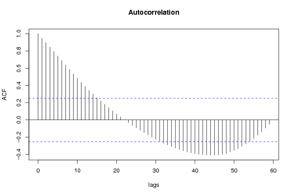
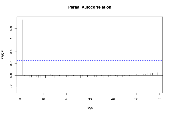
Title produced by software

(Partial) Autocorrelation Function

Date of computation

Mon, 08 Dec 2008 11:21:00 -0700

Cite this page as follows

Statistical Computations at FreeStatistics.org, Office for Research Development and Education, URL https://freestatistics.org/blog/index.php?v=date/2008/Dec/08/t1228760500kitj9bkppjti7g8.htm/, Retrieved Thu, 16 May 2024 21:54:38 +0000

Statistical Computations at FreeStatistics.org, Office for Research Development and Education, URL https://freestatistics.org/blog/index.php?pk=30642, Retrieved Thu, 16 May 2024 21:54:38 +0000

QR Codes:

Paste this QR Code to cite your computation.

Original text written by user:

IsPrivate?

No (this computation is public)

User-defined keywords

Estimated Impact

188

Family? (F = Feedback message, R = changed R code, M = changed R Module, P = changed Parameters, D = changed Data)

-     [Univariate Data Series] [data set] [2008-12-01 19:54:57] [b98453cac15ba1066b407e146608df68]
- RMP   [(Partial) Autocorrelation Function] [ACF] [2008-12-05 06:53:00] [c5a66f1c8528a963efc2b82a8519f117]
-    D    [(Partial) Autocorrelation Function] [ACF bouwvergunnin...] [2008-12-05 13:00:50] [c5a66f1c8528a963efc2b82a8519f117]
-    D        [(Partial) Autocorrelation Function] [ACF - woninghuur] [2008-12-08 18:21:00] [b4fc5040f26b33db57f84cfb8d1d2b82] [Current]

Feedback Forum

Post a new message

Dataseries X:

Download CSV

Histogram

Boxplots

Summary of computational transaction
Raw Input	view raw input (R code)
Raw Output	view raw output of R engine
Computing time	2 seconds
R Server	'Sir Ronald Aylmer Fisher' @ 193.190.124.24

\begin{tabular}{lllllllll}
\hline
Summary of computational transaction \tabularnewline
Raw Input & view raw input (R code)  \tabularnewline
Raw Output & view raw output of R engine  \tabularnewline
Computing time & 2 seconds \tabularnewline
R Server & 'Sir Ronald Aylmer Fisher' @ 193.190.124.24 \tabularnewline
\hline
\end{tabular}
%Source: https://freestatistics.org/blog/index.php?pk=30642&T=0

[TABLE]
[ROW][C]Summary of computational transaction[/C][/ROW]
[ROW][C]Raw Input[/C][C]view raw input (R code) [/C][/ROW]
[ROW][C]Raw Output[/C][C]view raw output of R engine [/C][/ROW]
[ROW][C]Computing time[/C][C]2 seconds[/C][/ROW]
[ROW][C]R Server[/C][C]'Sir Ronald Aylmer Fisher' @ 193.190.124.24[/C][/ROW]
[/TABLE]
Source: https://freestatistics.org/blog/index.php?pk=30642&T=0

Globally Unique Identifier (entire table): ba.freestatistics.org/blog/index.php?pk=30642&T=0

As an alternative you can also use a QR Code:

The GUIDs for individual cells are displayed in the table below:

Summary of computational transaction
Raw Input	view raw input (R code)
Raw Output	view raw output of R engine
Computing time	2 seconds
R Server	'Sir Ronald Aylmer Fisher' @ 193.190.124.24

Autocorrelation Function
Time lag k	ACF(k)	T-STAT	P-value
1	0.947985	7.3431	0
2	0.897377	6.9511	0
3	0.846028	6.5533	0
4	0.794216	6.152	0
5	0.742167	5.7488	0
6	0.689661	5.3421	1e-06
7	0.638161	4.9432	3e-06
8	0.586354	4.5419	1.4e-05
9	0.534461	4.1399	5.5e-05
10	0.485192	3.7583	0.000195
11	0.434913	3.3688	0.000662
12	0.386158	2.9912	0.002014
13	0.342605	2.6538	0.005087
14	0.300871	2.3305	0.011579
15	0.258865	2.0052	0.024732
16	0.219179	1.6978	0.047368
17	0.181457	1.4056	0.082506
18	0.143102	1.1085	0.136043
19	0.106163	0.8223	0.207072
20	0.069869	0.5412	0.295187
21	0.035267	0.2732	0.392828
22	0.000612	0.0047	0.498117
23	-0.031444	-0.2436	0.4042
24	-0.062816	-0.4866	0.314168
25	-0.091516	-0.7089	0.240571
26	-0.121242	-0.9391	0.175712
27	-0.148708	-1.1519	0.126968
28	-0.175309	-1.3579	0.089784
29	-0.200604	-1.5539	0.062737
30	-0.224238	-1.7369	0.043765
31	-0.247939	-1.9205	0.029774
32	-0.269816	-2.09	0.020433
33	-0.29029	-2.2486	0.014112
34	-0.309695	-2.3989	0.009785
35	-0.326476	-2.5289	0.007045
36	-0.34404	-2.6649	0.004939
37	-0.358657	-2.7781	0.003643
38	-0.372002	-2.8815	0.002741
39	-0.382097	-2.9597	0.002202
40	-0.391541	-3.0329	0.001788
41	-0.398247	-3.0848	0.001539
42	-0.403668	-3.1268	0.001362
43	-0.406703	-3.1503	0.001272
44	-0.409121	-3.169	0.001204
45	-0.408574	-3.1648	0.001219
46	-0.404224	-3.1311	0.001345
47	-0.398707	-3.0884	0.001523
48	-0.390065	-3.0214	0.001847
49	-0.374364	-2.8998	0.002605
50	-0.354727	-2.7477	0.003957
51	-0.333831	-2.5858	0.00608
52	-0.307966	-2.3855	0.010115
53	-0.279693	-2.1665	0.017128
54	-0.249035	-1.929	0.029231
55	-0.214366	-1.6605	0.051019
56	-0.177284	-1.3732	0.087394
57	-0.137391	-1.0642	0.145745
58	-0.094662	-0.7332	0.233132
59	-0.049603	-0.3842	0.351087
60	NA	NA	NA

\begin{tabular}{lllllllll}
\hline
Autocorrelation Function \tabularnewline
Time lag k & ACF(k) & T-STAT & P-value \tabularnewline
1 & 0.947985 & 7.3431 & 0 \tabularnewline
2 & 0.897377 & 6.9511 & 0 \tabularnewline
3 & 0.846028 & 6.5533 & 0 \tabularnewline
4 & 0.794216 & 6.152 & 0 \tabularnewline
5 & 0.742167 & 5.7488 & 0 \tabularnewline
6 & 0.689661 & 5.3421 & 1e-06 \tabularnewline
7 & 0.638161 & 4.9432 & 3e-06 \tabularnewline
8 & 0.586354 & 4.5419 & 1.4e-05 \tabularnewline
9 & 0.534461 & 4.1399 & 5.5e-05 \tabularnewline
10 & 0.485192 & 3.7583 & 0.000195 \tabularnewline
11 & 0.434913 & 3.3688 & 0.000662 \tabularnewline
12 & 0.386158 & 2.9912 & 0.002014 \tabularnewline
13 & 0.342605 & 2.6538 & 0.005087 \tabularnewline
14 & 0.300871 & 2.3305 & 0.011579 \tabularnewline
15 & 0.258865 & 2.0052 & 0.024732 \tabularnewline
16 & 0.219179 & 1.6978 & 0.047368 \tabularnewline
17 & 0.181457 & 1.4056 & 0.082506 \tabularnewline
18 & 0.143102 & 1.1085 & 0.136043 \tabularnewline
19 & 0.106163 & 0.8223 & 0.207072 \tabularnewline
20 & 0.069869 & 0.5412 & 0.295187 \tabularnewline
21 & 0.035267 & 0.2732 & 0.392828 \tabularnewline
22 & 0.000612 & 0.0047 & 0.498117 \tabularnewline
23 & -0.031444 & -0.2436 & 0.4042 \tabularnewline
24 & -0.062816 & -0.4866 & 0.314168 \tabularnewline
25 & -0.091516 & -0.7089 & 0.240571 \tabularnewline
26 & -0.121242 & -0.9391 & 0.175712 \tabularnewline
27 & -0.148708 & -1.1519 & 0.126968 \tabularnewline
28 & -0.175309 & -1.3579 & 0.089784 \tabularnewline
29 & -0.200604 & -1.5539 & 0.062737 \tabularnewline
30 & -0.224238 & -1.7369 & 0.043765 \tabularnewline
31 & -0.247939 & -1.9205 & 0.029774 \tabularnewline
32 & -0.269816 & -2.09 & 0.020433 \tabularnewline
33 & -0.29029 & -2.2486 & 0.014112 \tabularnewline
34 & -0.309695 & -2.3989 & 0.009785 \tabularnewline
35 & -0.326476 & -2.5289 & 0.007045 \tabularnewline
36 & -0.34404 & -2.6649 & 0.004939 \tabularnewline
37 & -0.358657 & -2.7781 & 0.003643 \tabularnewline
38 & -0.372002 & -2.8815 & 0.002741 \tabularnewline
39 & -0.382097 & -2.9597 & 0.002202 \tabularnewline
40 & -0.391541 & -3.0329 & 0.001788 \tabularnewline
41 & -0.398247 & -3.0848 & 0.001539 \tabularnewline
42 & -0.403668 & -3.1268 & 0.001362 \tabularnewline
43 & -0.406703 & -3.1503 & 0.001272 \tabularnewline
44 & -0.409121 & -3.169 & 0.001204 \tabularnewline
45 & -0.408574 & -3.1648 & 0.001219 \tabularnewline
46 & -0.404224 & -3.1311 & 0.001345 \tabularnewline
47 & -0.398707 & -3.0884 & 0.001523 \tabularnewline
48 & -0.390065 & -3.0214 & 0.001847 \tabularnewline
49 & -0.374364 & -2.8998 & 0.002605 \tabularnewline
50 & -0.354727 & -2.7477 & 0.003957 \tabularnewline
51 & -0.333831 & -2.5858 & 0.00608 \tabularnewline
52 & -0.307966 & -2.3855 & 0.010115 \tabularnewline
53 & -0.279693 & -2.1665 & 0.017128 \tabularnewline
54 & -0.249035 & -1.929 & 0.029231 \tabularnewline
55 & -0.214366 & -1.6605 & 0.051019 \tabularnewline
56 & -0.177284 & -1.3732 & 0.087394 \tabularnewline
57 & -0.137391 & -1.0642 & 0.145745 \tabularnewline
58 & -0.094662 & -0.7332 & 0.233132 \tabularnewline
59 & -0.049603 & -0.3842 & 0.351087 \tabularnewline
60 & NA & NA & NA \tabularnewline
\hline
\end{tabular}
%Source: https://freestatistics.org/blog/index.php?pk=30642&T=1

[TABLE]
[ROW][C]Autocorrelation Function[/C][/ROW]
[ROW][C]Time lag k[/C][C]ACF(k)[/C][C]T-STAT[/C][C]P-value[/C][/ROW]
[ROW][C]1[/C][C]0.947985[/C][C]7.3431[/C][C]0[/C][/ROW]
[ROW][C]2[/C][C]0.897377[/C][C]6.9511[/C][C]0[/C][/ROW]
[ROW][C]3[/C][C]0.846028[/C][C]6.5533[/C][C]0[/C][/ROW]
[ROW][C]4[/C][C]0.794216[/C][C]6.152[/C][C]0[/C][/ROW]
[ROW][C]5[/C][C]0.742167[/C][C]5.7488[/C][C]0[/C][/ROW]
[ROW][C]6[/C][C]0.689661[/C][C]5.3421[/C][C]1e-06[/C][/ROW]
[ROW][C]7[/C][C]0.638161[/C][C]4.9432[/C][C]3e-06[/C][/ROW]
[ROW][C]8[/C][C]0.586354[/C][C]4.5419[/C][C]1.4e-05[/C][/ROW]
[ROW][C]9[/C][C]0.534461[/C][C]4.1399[/C][C]5.5e-05[/C][/ROW]
[ROW][C]10[/C][C]0.485192[/C][C]3.7583[/C][C]0.000195[/C][/ROW]
[ROW][C]11[/C][C]0.434913[/C][C]3.3688[/C][C]0.000662[/C][/ROW]
[ROW][C]12[/C][C]0.386158[/C][C]2.9912[/C][C]0.002014[/C][/ROW]
[ROW][C]13[/C][C]0.342605[/C][C]2.6538[/C][C]0.005087[/C][/ROW]
[ROW][C]14[/C][C]0.300871[/C][C]2.3305[/C][C]0.011579[/C][/ROW]
[ROW][C]15[/C][C]0.258865[/C][C]2.0052[/C][C]0.024732[/C][/ROW]
[ROW][C]16[/C][C]0.219179[/C][C]1.6978[/C][C]0.047368[/C][/ROW]
[ROW][C]17[/C][C]0.181457[/C][C]1.4056[/C][C]0.082506[/C][/ROW]
[ROW][C]18[/C][C]0.143102[/C][C]1.1085[/C][C]0.136043[/C][/ROW]
[ROW][C]19[/C][C]0.106163[/C][C]0.8223[/C][C]0.207072[/C][/ROW]
[ROW][C]20[/C][C]0.069869[/C][C]0.5412[/C][C]0.295187[/C][/ROW]
[ROW][C]21[/C][C]0.035267[/C][C]0.2732[/C][C]0.392828[/C][/ROW]
[ROW][C]22[/C][C]0.000612[/C][C]0.0047[/C][C]0.498117[/C][/ROW]
[ROW][C]23[/C][C]-0.031444[/C][C]-0.2436[/C][C]0.4042[/C][/ROW]
[ROW][C]24[/C][C]-0.062816[/C][C]-0.4866[/C][C]0.314168[/C][/ROW]
[ROW][C]25[/C][C]-0.091516[/C][C]-0.7089[/C][C]0.240571[/C][/ROW]
[ROW][C]26[/C][C]-0.121242[/C][C]-0.9391[/C][C]0.175712[/C][/ROW]
[ROW][C]27[/C][C]-0.148708[/C][C]-1.1519[/C][C]0.126968[/C][/ROW]
[ROW][C]28[/C][C]-0.175309[/C][C]-1.3579[/C][C]0.089784[/C][/ROW]
[ROW][C]29[/C][C]-0.200604[/C][C]-1.5539[/C][C]0.062737[/C][/ROW]
[ROW][C]30[/C][C]-0.224238[/C][C]-1.7369[/C][C]0.043765[/C][/ROW]
[ROW][C]31[/C][C]-0.247939[/C][C]-1.9205[/C][C]0.029774[/C][/ROW]
[ROW][C]32[/C][C]-0.269816[/C][C]-2.09[/C][C]0.020433[/C][/ROW]
[ROW][C]33[/C][C]-0.29029[/C][C]-2.2486[/C][C]0.014112[/C][/ROW]
[ROW][C]34[/C][C]-0.309695[/C][C]-2.3989[/C][C]0.009785[/C][/ROW]
[ROW][C]35[/C][C]-0.326476[/C][C]-2.5289[/C][C]0.007045[/C][/ROW]
[ROW][C]36[/C][C]-0.34404[/C][C]-2.6649[/C][C]0.004939[/C][/ROW]
[ROW][C]37[/C][C]-0.358657[/C][C]-2.7781[/C][C]0.003643[/C][/ROW]
[ROW][C]38[/C][C]-0.372002[/C][C]-2.8815[/C][C]0.002741[/C][/ROW]
[ROW][C]39[/C][C]-0.382097[/C][C]-2.9597[/C][C]0.002202[/C][/ROW]
[ROW][C]40[/C][C]-0.391541[/C][C]-3.0329[/C][C]0.001788[/C][/ROW]
[ROW][C]41[/C][C]-0.398247[/C][C]-3.0848[/C][C]0.001539[/C][/ROW]
[ROW][C]42[/C][C]-0.403668[/C][C]-3.1268[/C][C]0.001362[/C][/ROW]
[ROW][C]43[/C][C]-0.406703[/C][C]-3.1503[/C][C]0.001272[/C][/ROW]
[ROW][C]44[/C][C]-0.409121[/C][C]-3.169[/C][C]0.001204[/C][/ROW]
[ROW][C]45[/C][C]-0.408574[/C][C]-3.1648[/C][C]0.001219[/C][/ROW]
[ROW][C]46[/C][C]-0.404224[/C][C]-3.1311[/C][C]0.001345[/C][/ROW]
[ROW][C]47[/C][C]-0.398707[/C][C]-3.0884[/C][C]0.001523[/C][/ROW]
[ROW][C]48[/C][C]-0.390065[/C][C]-3.0214[/C][C]0.001847[/C][/ROW]
[ROW][C]49[/C][C]-0.374364[/C][C]-2.8998[/C][C]0.002605[/C][/ROW]
[ROW][C]50[/C][C]-0.354727[/C][C]-2.7477[/C][C]0.003957[/C][/ROW]
[ROW][C]51[/C][C]-0.333831[/C][C]-2.5858[/C][C]0.00608[/C][/ROW]
[ROW][C]52[/C][C]-0.307966[/C][C]-2.3855[/C][C]0.010115[/C][/ROW]
[ROW][C]53[/C][C]-0.279693[/C][C]-2.1665[/C][C]0.017128[/C][/ROW]
[ROW][C]54[/C][C]-0.249035[/C][C]-1.929[/C][C]0.029231[/C][/ROW]
[ROW][C]55[/C][C]-0.214366[/C][C]-1.6605[/C][C]0.051019[/C][/ROW]
[ROW][C]56[/C][C]-0.177284[/C][C]-1.3732[/C][C]0.087394[/C][/ROW]
[ROW][C]57[/C][C]-0.137391[/C][C]-1.0642[/C][C]0.145745[/C][/ROW]
[ROW][C]58[/C][C]-0.094662[/C][C]-0.7332[/C][C]0.233132[/C][/ROW]
[ROW][C]59[/C][C]-0.049603[/C][C]-0.3842[/C][C]0.351087[/C][/ROW]
[ROW][C]60[/C][C]NA[/C][C]NA[/C][C]NA[/C][/ROW]
[/TABLE]
Source: https://freestatistics.org/blog/index.php?pk=30642&T=1

Globally Unique Identifier (entire table): ba.freestatistics.org/blog/index.php?pk=30642&T=1

As an alternative you can also use a QR Code:

The GUIDs for individual cells are displayed in the table below:

Autocorrelation Function
Time lag k	ACF(k)	T-STAT	P-value
1	0.947985	7.3431	0
2	0.897377	6.9511	0
3	0.846028	6.5533	0
4	0.794216	6.152	0
5	0.742167	5.7488	0
6	0.689661	5.3421	1e-06
7	0.638161	4.9432	3e-06
8	0.586354	4.5419	1.4e-05
9	0.534461	4.1399	5.5e-05
10	0.485192	3.7583	0.000195
11	0.434913	3.3688	0.000662
12	0.386158	2.9912	0.002014
13	0.342605	2.6538	0.005087
14	0.300871	2.3305	0.011579
15	0.258865	2.0052	0.024732
16	0.219179	1.6978	0.047368
17	0.181457	1.4056	0.082506
18	0.143102	1.1085	0.136043
19	0.106163	0.8223	0.207072
20	0.069869	0.5412	0.295187
21	0.035267	0.2732	0.392828
22	0.000612	0.0047	0.498117
23	-0.031444	-0.2436	0.4042
24	-0.062816	-0.4866	0.314168
25	-0.091516	-0.7089	0.240571
26	-0.121242	-0.9391	0.175712
27	-0.148708	-1.1519	0.126968
28	-0.175309	-1.3579	0.089784
29	-0.200604	-1.5539	0.062737
30	-0.224238	-1.7369	0.043765
31	-0.247939	-1.9205	0.029774
32	-0.269816	-2.09	0.020433
33	-0.29029	-2.2486	0.014112
34	-0.309695	-2.3989	0.009785
35	-0.326476	-2.5289	0.007045
36	-0.34404	-2.6649	0.004939
37	-0.358657	-2.7781	0.003643
38	-0.372002	-2.8815	0.002741
39	-0.382097	-2.9597	0.002202
40	-0.391541	-3.0329	0.001788
41	-0.398247	-3.0848	0.001539
42	-0.403668	-3.1268	0.001362
43	-0.406703	-3.1503	0.001272
44	-0.409121	-3.169	0.001204
45	-0.408574	-3.1648	0.001219
46	-0.404224	-3.1311	0.001345
47	-0.398707	-3.0884	0.001523
48	-0.390065	-3.0214	0.001847
49	-0.374364	-2.8998	0.002605
50	-0.354727	-2.7477	0.003957
51	-0.333831	-2.5858	0.00608
52	-0.307966	-2.3855	0.010115
53	-0.279693	-2.1665	0.017128
54	-0.249035	-1.929	0.029231
55	-0.214366	-1.6605	0.051019
56	-0.177284	-1.3732	0.087394
57	-0.137391	-1.0642	0.145745
58	-0.094662	-0.7332	0.233132
59	-0.049603	-0.3842	0.351087
60	NA	NA	NA

Partial Autocorrelation Function
Time lag k	PACF(k)	T-STAT	P-value
1	0.947985	7.3431	0
2	-0.012806	-0.0992	0.460658
3	-0.033816	-0.2619	0.397134
4	-0.032577	-0.2523	0.400819
5	-0.031301	-0.2425	0.404625
6	-0.034395	-0.2664	0.395412
7	-0.02118	-0.1641	0.435117
8	-0.034139	-0.2644	0.396174
9	-0.033677	-0.2609	0.397546
10	-0.007774	-0.0602	0.476092
11	-0.042563	-0.3297	0.371392
12	-0.020528	-0.159	0.437098
13	0.017005	0.1317	0.447824
14	-0.013679	-0.106	0.457986
15	-0.035966	-0.2786	0.390757
16	-0.011138	-0.0863	0.465768
17	-0.014228	-0.1102	0.456304
18	-0.039814	-0.3084	0.379424
19	-0.020101	-0.1557	0.438394
20	-0.028964	-0.2244	0.411621
21	-0.018875	-0.1462	0.442124
22	-0.033772	-0.2616	0.397263
23	-0.011106	-0.086	0.465865
24	-0.028694	-0.2223	0.412433
25	-0.006322	-0.049	0.480552
26	-0.044036	-0.3411	0.367109
27	-0.016285	-0.1261	0.45002
28	-0.025686	-0.199	0.421481
29	-0.022567	-0.1748	0.430913
30	-0.021267	-0.1647	0.434853
31	-0.037403	-0.2897	0.386515
32	-0.019128	-0.1482	0.441356
33	-0.023587	-0.1827	0.427825
34	-0.026489	-0.2052	0.419062
35	-0.011771	-0.0912	0.463828
36	-0.042636	-0.3303	0.371178
37	-0.009439	-0.0731	0.470979
38	-0.024577	-0.1904	0.424829
39	-0.003598	-0.0279	0.48893
40	-0.028733	-0.2226	0.412314
41	-0.007218	-0.0559	0.477798
42	-0.022179	-0.1718	0.432088
43	-0.009329	-0.0723	0.471317
44	-0.0263	-0.2037	0.41963
45	-0.002241	-0.0174	0.493105
46	0.008237	0.0638	0.47467
47	-0.01368	-0.106	0.457981
48	0.004069	0.0315	0.48748
49	0.048696	0.3772	0.353678
50	0.025338	0.1963	0.422531
51	0.001099	0.0085	0.496618
52	0.039452	0.3056	0.380487
53	0.02012	0.1558	0.438337
54	0.022917	0.1775	0.429851
55	0.044299	0.3431	0.366346
56	0.031019	0.2403	0.405469
57	0.042299	0.3276	0.372158
58	0.049323	0.3821	0.351886
59	0.047646	0.3691	0.35669
60	NA	NA	NA

\begin{tabular}{lllllllll}
\hline
Partial Autocorrelation Function \tabularnewline
Time lag k & PACF(k) & T-STAT & P-value \tabularnewline
1 & 0.947985 & 7.3431 & 0 \tabularnewline
2 & -0.012806 & -0.0992 & 0.460658 \tabularnewline
3 & -0.033816 & -0.2619 & 0.397134 \tabularnewline
4 & -0.032577 & -0.2523 & 0.400819 \tabularnewline
5 & -0.031301 & -0.2425 & 0.404625 \tabularnewline
6 & -0.034395 & -0.2664 & 0.395412 \tabularnewline
7 & -0.02118 & -0.1641 & 0.435117 \tabularnewline
8 & -0.034139 & -0.2644 & 0.396174 \tabularnewline
9 & -0.033677 & -0.2609 & 0.397546 \tabularnewline
10 & -0.007774 & -0.0602 & 0.476092 \tabularnewline
11 & -0.042563 & -0.3297 & 0.371392 \tabularnewline
12 & -0.020528 & -0.159 & 0.437098 \tabularnewline
13 & 0.017005 & 0.1317 & 0.447824 \tabularnewline
14 & -0.013679 & -0.106 & 0.457986 \tabularnewline
15 & -0.035966 & -0.2786 & 0.390757 \tabularnewline
16 & -0.011138 & -0.0863 & 0.465768 \tabularnewline
17 & -0.014228 & -0.1102 & 0.456304 \tabularnewline
18 & -0.039814 & -0.3084 & 0.379424 \tabularnewline
19 & -0.020101 & -0.1557 & 0.438394 \tabularnewline
20 & -0.028964 & -0.2244 & 0.411621 \tabularnewline
21 & -0.018875 & -0.1462 & 0.442124 \tabularnewline
22 & -0.033772 & -0.2616 & 0.397263 \tabularnewline
23 & -0.011106 & -0.086 & 0.465865 \tabularnewline
24 & -0.028694 & -0.2223 & 0.412433 \tabularnewline
25 & -0.006322 & -0.049 & 0.480552 \tabularnewline
26 & -0.044036 & -0.3411 & 0.367109 \tabularnewline
27 & -0.016285 & -0.1261 & 0.45002 \tabularnewline
28 & -0.025686 & -0.199 & 0.421481 \tabularnewline
29 & -0.022567 & -0.1748 & 0.430913 \tabularnewline
30 & -0.021267 & -0.1647 & 0.434853 \tabularnewline
31 & -0.037403 & -0.2897 & 0.386515 \tabularnewline
32 & -0.019128 & -0.1482 & 0.441356 \tabularnewline
33 & -0.023587 & -0.1827 & 0.427825 \tabularnewline
34 & -0.026489 & -0.2052 & 0.419062 \tabularnewline
35 & -0.011771 & -0.0912 & 0.463828 \tabularnewline
36 & -0.042636 & -0.3303 & 0.371178 \tabularnewline
37 & -0.009439 & -0.0731 & 0.470979 \tabularnewline
38 & -0.024577 & -0.1904 & 0.424829 \tabularnewline
39 & -0.003598 & -0.0279 & 0.48893 \tabularnewline
40 & -0.028733 & -0.2226 & 0.412314 \tabularnewline
41 & -0.007218 & -0.0559 & 0.477798 \tabularnewline
42 & -0.022179 & -0.1718 & 0.432088 \tabularnewline
43 & -0.009329 & -0.0723 & 0.471317 \tabularnewline
44 & -0.0263 & -0.2037 & 0.41963 \tabularnewline
45 & -0.002241 & -0.0174 & 0.493105 \tabularnewline
46 & 0.008237 & 0.0638 & 0.47467 \tabularnewline
47 & -0.01368 & -0.106 & 0.457981 \tabularnewline
48 & 0.004069 & 0.0315 & 0.48748 \tabularnewline
49 & 0.048696 & 0.3772 & 0.353678 \tabularnewline
50 & 0.025338 & 0.1963 & 0.422531 \tabularnewline
51 & 0.001099 & 0.0085 & 0.496618 \tabularnewline
52 & 0.039452 & 0.3056 & 0.380487 \tabularnewline
53 & 0.02012 & 0.1558 & 0.438337 \tabularnewline
54 & 0.022917 & 0.1775 & 0.429851 \tabularnewline
55 & 0.044299 & 0.3431 & 0.366346 \tabularnewline
56 & 0.031019 & 0.2403 & 0.405469 \tabularnewline
57 & 0.042299 & 0.3276 & 0.372158 \tabularnewline
58 & 0.049323 & 0.3821 & 0.351886 \tabularnewline
59 & 0.047646 & 0.3691 & 0.35669 \tabularnewline
60 & NA & NA & NA \tabularnewline
\hline
\end{tabular}
%Source: https://freestatistics.org/blog/index.php?pk=30642&T=2

[TABLE]
[ROW][C]Partial Autocorrelation Function[/C][/ROW]
[ROW][C]Time lag k[/C][C]PACF(k)[/C][C]T-STAT[/C][C]P-value[/C][/ROW]
[ROW][C]1[/C][C]0.947985[/C][C]7.3431[/C][C]0[/C][/ROW]
[ROW][C]2[/C][C]-0.012806[/C][C]-0.0992[/C][C]0.460658[/C][/ROW]
[ROW][C]3[/C][C]-0.033816[/C][C]-0.2619[/C][C]0.397134[/C][/ROW]
[ROW][C]4[/C][C]-0.032577[/C][C]-0.2523[/C][C]0.400819[/C][/ROW]
[ROW][C]5[/C][C]-0.031301[/C][C]-0.2425[/C][C]0.404625[/C][/ROW]
[ROW][C]6[/C][C]-0.034395[/C][C]-0.2664[/C][C]0.395412[/C][/ROW]
[ROW][C]7[/C][C]-0.02118[/C][C]-0.1641[/C][C]0.435117[/C][/ROW]
[ROW][C]8[/C][C]-0.034139[/C][C]-0.2644[/C][C]0.396174[/C][/ROW]
[ROW][C]9[/C][C]-0.033677[/C][C]-0.2609[/C][C]0.397546[/C][/ROW]
[ROW][C]10[/C][C]-0.007774[/C][C]-0.0602[/C][C]0.476092[/C][/ROW]
[ROW][C]11[/C][C]-0.042563[/C][C]-0.3297[/C][C]0.371392[/C][/ROW]
[ROW][C]12[/C][C]-0.020528[/C][C]-0.159[/C][C]0.437098[/C][/ROW]
[ROW][C]13[/C][C]0.017005[/C][C]0.1317[/C][C]0.447824[/C][/ROW]
[ROW][C]14[/C][C]-0.013679[/C][C]-0.106[/C][C]0.457986[/C][/ROW]
[ROW][C]15[/C][C]-0.035966[/C][C]-0.2786[/C][C]0.390757[/C][/ROW]
[ROW][C]16[/C][C]-0.011138[/C][C]-0.0863[/C][C]0.465768[/C][/ROW]
[ROW][C]17[/C][C]-0.014228[/C][C]-0.1102[/C][C]0.456304[/C][/ROW]
[ROW][C]18[/C][C]-0.039814[/C][C]-0.3084[/C][C]0.379424[/C][/ROW]
[ROW][C]19[/C][C]-0.020101[/C][C]-0.1557[/C][C]0.438394[/C][/ROW]
[ROW][C]20[/C][C]-0.028964[/C][C]-0.2244[/C][C]0.411621[/C][/ROW]
[ROW][C]21[/C][C]-0.018875[/C][C]-0.1462[/C][C]0.442124[/C][/ROW]
[ROW][C]22[/C][C]-0.033772[/C][C]-0.2616[/C][C]0.397263[/C][/ROW]
[ROW][C]23[/C][C]-0.011106[/C][C]-0.086[/C][C]0.465865[/C][/ROW]
[ROW][C]24[/C][C]-0.028694[/C][C]-0.2223[/C][C]0.412433[/C][/ROW]
[ROW][C]25[/C][C]-0.006322[/C][C]-0.049[/C][C]0.480552[/C][/ROW]
[ROW][C]26[/C][C]-0.044036[/C][C]-0.3411[/C][C]0.367109[/C][/ROW]
[ROW][C]27[/C][C]-0.016285[/C][C]-0.1261[/C][C]0.45002[/C][/ROW]
[ROW][C]28[/C][C]-0.025686[/C][C]-0.199[/C][C]0.421481[/C][/ROW]
[ROW][C]29[/C][C]-0.022567[/C][C]-0.1748[/C][C]0.430913[/C][/ROW]
[ROW][C]30[/C][C]-0.021267[/C][C]-0.1647[/C][C]0.434853[/C][/ROW]
[ROW][C]31[/C][C]-0.037403[/C][C]-0.2897[/C][C]0.386515[/C][/ROW]
[ROW][C]32[/C][C]-0.019128[/C][C]-0.1482[/C][C]0.441356[/C][/ROW]
[ROW][C]33[/C][C]-0.023587[/C][C]-0.1827[/C][C]0.427825[/C][/ROW]
[ROW][C]34[/C][C]-0.026489[/C][C]-0.2052[/C][C]0.419062[/C][/ROW]
[ROW][C]35[/C][C]-0.011771[/C][C]-0.0912[/C][C]0.463828[/C][/ROW]
[ROW][C]36[/C][C]-0.042636[/C][C]-0.3303[/C][C]0.371178[/C][/ROW]
[ROW][C]37[/C][C]-0.009439[/C][C]-0.0731[/C][C]0.470979[/C][/ROW]
[ROW][C]38[/C][C]-0.024577[/C][C]-0.1904[/C][C]0.424829[/C][/ROW]
[ROW][C]39[/C][C]-0.003598[/C][C]-0.0279[/C][C]0.48893[/C][/ROW]
[ROW][C]40[/C][C]-0.028733[/C][C]-0.2226[/C][C]0.412314[/C][/ROW]
[ROW][C]41[/C][C]-0.007218[/C][C]-0.0559[/C][C]0.477798[/C][/ROW]
[ROW][C]42[/C][C]-0.022179[/C][C]-0.1718[/C][C]0.432088[/C][/ROW]
[ROW][C]43[/C][C]-0.009329[/C][C]-0.0723[/C][C]0.471317[/C][/ROW]
[ROW][C]44[/C][C]-0.0263[/C][C]-0.2037[/C][C]0.41963[/C][/ROW]
[ROW][C]45[/C][C]-0.002241[/C][C]-0.0174[/C][C]0.493105[/C][/ROW]
[ROW][C]46[/C][C]0.008237[/C][C]0.0638[/C][C]0.47467[/C][/ROW]
[ROW][C]47[/C][C]-0.01368[/C][C]-0.106[/C][C]0.457981[/C][/ROW]
[ROW][C]48[/C][C]0.004069[/C][C]0.0315[/C][C]0.48748[/C][/ROW]
[ROW][C]49[/C][C]0.048696[/C][C]0.3772[/C][C]0.353678[/C][/ROW]
[ROW][C]50[/C][C]0.025338[/C][C]0.1963[/C][C]0.422531[/C][/ROW]
[ROW][C]51[/C][C]0.001099[/C][C]0.0085[/C][C]0.496618[/C][/ROW]
[ROW][C]52[/C][C]0.039452[/C][C]0.3056[/C][C]0.380487[/C][/ROW]
[ROW][C]53[/C][C]0.02012[/C][C]0.1558[/C][C]0.438337[/C][/ROW]
[ROW][C]54[/C][C]0.022917[/C][C]0.1775[/C][C]0.429851[/C][/ROW]
[ROW][C]55[/C][C]0.044299[/C][C]0.3431[/C][C]0.366346[/C][/ROW]
[ROW][C]56[/C][C]0.031019[/C][C]0.2403[/C][C]0.405469[/C][/ROW]
[ROW][C]57[/C][C]0.042299[/C][C]0.3276[/C][C]0.372158[/C][/ROW]
[ROW][C]58[/C][C]0.049323[/C][C]0.3821[/C][C]0.351886[/C][/ROW]
[ROW][C]59[/C][C]0.047646[/C][C]0.3691[/C][C]0.35669[/C][/ROW]
[ROW][C]60[/C][C]NA[/C][C]NA[/C][C]NA[/C][/ROW]
[/TABLE]
Source: https://freestatistics.org/blog/index.php?pk=30642&T=2

Globally Unique Identifier (entire table): ba.freestatistics.org/blog/index.php?pk=30642&T=2

As an alternative you can also use a QR Code:

The GUIDs for individual cells are displayed in the table below:

Partial Autocorrelation Function
Time lag k	PACF(k)	T-STAT	P-value
1	0.947985	7.3431	0
2	-0.012806	-0.0992	0.460658
3	-0.033816	-0.2619	0.397134
4	-0.032577	-0.2523	0.400819
5	-0.031301	-0.2425	0.404625
6	-0.034395	-0.2664	0.395412
7	-0.02118	-0.1641	0.435117
8	-0.034139	-0.2644	0.396174
9	-0.033677	-0.2609	0.397546
10	-0.007774	-0.0602	0.476092
11	-0.042563	-0.3297	0.371392
12	-0.020528	-0.159	0.437098
13	0.017005	0.1317	0.447824
14	-0.013679	-0.106	0.457986
15	-0.035966	-0.2786	0.390757
16	-0.011138	-0.0863	0.465768
17	-0.014228	-0.1102	0.456304
18	-0.039814	-0.3084	0.379424
19	-0.020101	-0.1557	0.438394
20	-0.028964	-0.2244	0.411621
21	-0.018875	-0.1462	0.442124
22	-0.033772	-0.2616	0.397263
23	-0.011106	-0.086	0.465865
24	-0.028694	-0.2223	0.412433
25	-0.006322	-0.049	0.480552
26	-0.044036	-0.3411	0.367109
27	-0.016285	-0.1261	0.45002
28	-0.025686	-0.199	0.421481
29	-0.022567	-0.1748	0.430913
30	-0.021267	-0.1647	0.434853
31	-0.037403	-0.2897	0.386515
32	-0.019128	-0.1482	0.441356
33	-0.023587	-0.1827	0.427825
34	-0.026489	-0.2052	0.419062
35	-0.011771	-0.0912	0.463828
36	-0.042636	-0.3303	0.371178
37	-0.009439	-0.0731	0.470979
38	-0.024577	-0.1904	0.424829
39	-0.003598	-0.0279	0.48893
40	-0.028733	-0.2226	0.412314
41	-0.007218	-0.0559	0.477798
42	-0.022179	-0.1718	0.432088
43	-0.009329	-0.0723	0.471317
44	-0.0263	-0.2037	0.41963
45	-0.002241	-0.0174	0.493105
46	0.008237	0.0638	0.47467
47	-0.01368	-0.106	0.457981
48	0.004069	0.0315	0.48748
49	0.048696	0.3772	0.353678
50	0.025338	0.1963	0.422531
51	0.001099	0.0085	0.496618
52	0.039452	0.3056	0.380487
53	0.02012	0.1558	0.438337
54	0.022917	0.1775	0.429851
55	0.044299	0.3431	0.366346
56	0.031019	0.2403	0.405469
57	0.042299	0.3276	0.372158
58	0.049323	0.3821	0.351886
59	0.047646	0.3691	0.35669
60	NA	NA	NA

Figure 1

PNG link

Postscript link

PDF link

Figure 2

PNG link

Postscript link

PDF link

Parameters (Session):

par1 = 60 ; par2 = 1 ; par3 = 0 ; par4 = 0 ; par5 = 12 ;

Parameters (R input):

par1 = 60 ; par2 = 1 ; par3 = 0 ; par4 = 0 ; par5 = 12 ;

R code (references can be found in the software module):

if (par1 == 'Default') {
par1 = 10*log10(length(x))
} else {
par1 <- as.numeric(par1)
}
par2 <- as.numeric(par2)
par3 <- as.numeric(par3)
par4 <- as.numeric(par4)
par5 <- as.numeric(par5)
if (par2 == 0) {
x <- log(x)
} else {
x <- (x ^ par2 - 1) / par2
}
if (par3 > 0) x <- diff(x,lag=1,difference=par3)
if (par4 > 0) x <- diff(x,lag=par5,difference=par4)
bitmap(file='pic1.png')
racf <- acf(x,par1,main='Autocorrelation',xlab='lags',ylab='ACF')
dev.off()
bitmap(file='pic2.png')
rpacf <- pacf(x,par1,main='Partial Autocorrelation',xlab='lags',ylab='PACF')
dev.off()
(myacf <- c(racf$acf))
(mypacf <- c(rpacf$acf))
lengthx <- length(x)
sqrtn <- sqrt(lengthx)
load(file='createtable')
a<-table.start()
a<-table.row.start(a)
a<-table.element(a,'Autocorrelation Function',4,TRUE)
a<-table.row.end(a)
a<-table.row.start(a)
a<-table.element(a,'Time lag k',header=TRUE)
a<-table.element(a,hyperlink('basics.htm','ACF(k)','click here for more information about the Autocorrelation Function'),header=TRUE)
a<-table.element(a,'T-STAT',header=TRUE)
a<-table.element(a,'P-value',header=TRUE)
a<-table.row.end(a)
for (i in 2:(par1+1)) {
a<-table.row.start(a)
a<-table.element(a,i-1,header=TRUE)
a<-table.element(a,round(myacf[i],6))
mytstat <- myacf[i]*sqrtn
a<-table.element(a,round(mytstat,4))
a<-table.element(a,round(1-pt(abs(mytstat),lengthx),6))
a<-table.row.end(a)
}
a<-table.end(a)
table.save(a,file='mytable.tab')
a<-table.start()
a<-table.row.start(a)
a<-table.element(a,'Partial Autocorrelation Function',4,TRUE)
a<-table.row.end(a)
a<-table.row.start(a)
a<-table.element(a,'Time lag k',header=TRUE)
a<-table.element(a,hyperlink('basics.htm','PACF(k)','click here for more information about the Partial Autocorrelation Function'),header=TRUE)
a<-table.element(a,'T-STAT',header=TRUE)
a<-table.element(a,'P-value',header=TRUE)
a<-table.row.end(a)
for (i in 1:par1) {
a<-table.row.start(a)
a<-table.element(a,i,header=TRUE)
a<-table.element(a,round(mypacf[i],6))
mytstat <- mypacf[i]*sqrtn
a<-table.element(a,round(mytstat,4))
a<-table.element(a,round(1-pt(abs(mytstat),lengthx),6))
a<-table.row.end(a)
}
a<-table.end(a)
table.save(a,file='mytable1.tab')

Free Statistics

Description of Statistical Computation

Tree of Dependent Computations

Dataset

Tables (Output of Computation)

Figures (Output of Computation)

Input Parameters & R Code