Repository of Reproducible Computations

Free Statistics

of Irreproducible Research!

Author's title

Author

*The author of this computation has been verified*

R Software Module

rwasp_autocorrelation.wasp

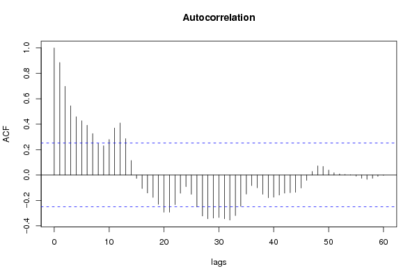
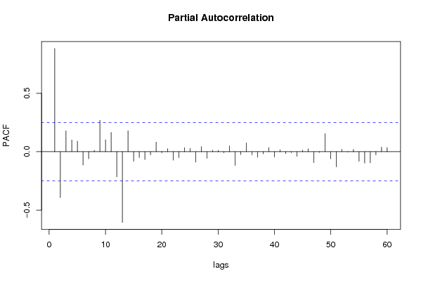
Title produced by software

(Partial) Autocorrelation Function

Date of computation

Mon, 08 Dec 2008 11:00:18 -0700

Cite this page as follows

Statistical Computations at FreeStatistics.org, Office for Research Development and Education, URL https://freestatistics.org/blog/index.php?v=date/2008/Dec/08/t1228759259pwjge0hm7cd90j5.htm/, Retrieved Thu, 16 May 2024 16:16:36 +0000

Statistical Computations at FreeStatistics.org, Office for Research Development and Education, URL https://freestatistics.org/blog/index.php?pk=30633, Retrieved Thu, 16 May 2024 16:16:36 +0000

QR Codes:

Paste this QR Code to cite your computation.

Original text written by user:

IsPrivate?

No (this computation is public)

User-defined keywords

Estimated Impact

210

Family? (F = Feedback message, R = changed R code, M = changed R Module, P = changed Parameters, D = changed Data)

F     [(Partial) Autocorrelation Function] [Unemployment - St...] [2008-12-08 17:24:07] [57850c80fd59ccfb28f882be994e814e]
F   P     [(Partial) Autocorrelation Function] [Unemployment - St...] [2008-12-08 18:00:18] [0831954c833179c36e9320daee0825b5] [Current]
F           [(Partial) Autocorrelation Function] [STEP 1 2] [2008-12-08 18:50:07] [547636b63517c1c2916a747d66b36ebf] 
-           [(Partial) Autocorrelation Function] [Step 2] [2008-12-08 20:48:25] [6816386b1f3c2f6c0c9f2aa1e5bc9362] 
F    D        [(Partial) Autocorrelation Function] [Step 2] [2008-12-08 21:55:57] [cf9c64468d04c2c4dd548cc66b4e3677] 
-   P           [(Partial) Autocorrelation Function] [Step 2.2] [2008-12-08 21:59:02] [cf9c64468d04c2c4dd548cc66b4e3677] 
-   P             [(Partial) Autocorrelation Function] [step 2.3] [2008-12-08 22:03:20] [cf9c64468d04c2c4dd548cc66b4e3677] 
F                   [(Partial) Autocorrelation Function] [Step 2_d=1, D=1] [2008-12-08 23:06:07] [6816386b1f3c2f6c0c9f2aa1e5bc9362] 
F                     [(Partial) Autocorrelation Function] [step 2 ; d and D=1] [2008-12-08 23:36:11] [73d6180dc45497329efd1b6934a84aba] 
F                     [(Partial) Autocorrelation Function] [] [2008-12-09 00:15:14] [74be16979710d4c4e7c6647856088456] 
-                       [(Partial) Autocorrelation Function] [] [2008-12-15 22:47:58] [74be16979710d4c4e7c6647856088456] 
F                 [(Partial) Autocorrelation Function] [Step 2_d=1, D=0] [2008-12-08 23:04:21] [6816386b1f3c2f6c0c9f2aa1e5bc9362] 
F                   [(Partial) Autocorrelation Function] [step 2; d=1 en D=0] [2008-12-08 23:34:56] [73d6180dc45497329efd1b6934a84aba] 
F                   [(Partial) Autocorrelation Function] [] [2008-12-09 00:14:04] [74be16979710d4c4e7c6647856088456] 
-                     [(Partial) Autocorrelation Function] [] [2008-12-15 22:46:23] [74be16979710d4c4e7c6647856088456] 
F               [(Partial) Autocorrelation Function] [Step 2_d&D = 0] [2008-12-08 23:01:09] [6816386b1f3c2f6c0c9f2aa1e5bc9362] 
F                 [(Partial) Autocorrelation Function] [step 2; d and D= 0] [2008-12-08 23:32:01] [73d6180dc45497329efd1b6934a84aba] 
F                 [(Partial) Autocorrelation Function] [] [2008-12-09 00:12:24] [74be16979710d4c4e7c6647856088456] 
-                   [(Partial) Autocorrelation Function] [] [2008-12-15 22:44:13] [74be16979710d4c4e7c6647856088456] 
-             [(Partial) Autocorrelation Function] [step 2] [2008-12-08 23:49:20] [73d6180dc45497329efd1b6934a84aba] 
-             [(Partial) Autocorrelation Function] [] [2008-12-09 00:26:02] [74be16979710d4c4e7c6647856088456] 
F    D      [(Partial) Autocorrelation Function] [] [2008-12-08 21:18:59] [4c8dfb519edec2da3492d7e6be9a5685] 

Feedback Forum

2008-12-14 23:54:00 [Bob Leysen] [reply] 
We zien een fluctuerende dalende trend van een niet-stationaire tijdreeks.  
 
De oorzaak van de gote pieken is dat d=0 en D=0  
 
In de volgende grafieken gaan de pieken geleidelijk weg, tot we komen aan een model met d=1 en D=1
2008-12-15 09:14:06 [Glenn De Maeyer] [reply] 
De student werkte stap 2 uit voor zijn eigen tijdreeksen. Dit werd correct uitgevoerd. 
De tweede stap diende ook uitgevoerd te worden op de tijdreeks unemployment data. 
Dit volgt hieronder. 
 
Variance reduction matrix 
 
http://www.freestatistics.org/blog/index.php?v=date/2008/Dec/15/t12293281189uokrv2hf06li3f.htm 
 
We noteren de kleinste waarde 795.483036989776 waar d = 1 en D = 1, dit wil zeggen dat we één maal gewoon en één maal seizonaal moeten differentiëren om de datareeks stationair te maken. 
 
Autocorrelation function 
 
http://www.freestatistics.org/blog/index.php?v=date/2008/Dec/15/t1229328245riclpjxysffnhqp.htm 
 
Wanneer we de grafiek analyseren merken we duidelijk een lange termijn trend op. Deze werken we weg door de parameters correct aan te passen.  
 
We voeren dus nu in de software de correcte waarden in. (Lambda= 0,5, d=1, D=1 lags=60) 
 
http://www.freestatistics.org/blog/index.php?v=date/2008/Dec/15/t1229328575r41j4a7qfnzz9pi.htm 
 
Op deze grafiek is de trend verdwenen. We vermoeden trouwens een conjunctuur, we vermoeden dus een AR proces. 
 
Cumulative periodogram 
 
http://www.freestatistics.org/blog/index.php?v=date/2008/Dec/15/t12293289767j1xpvxsk8gnjgi.htm 
 
We merken hier een afwijking op naar boven toe. Dit wijst er op dat er sprake is van een AR proces. AR is een goed proces wanneer we conjunctuur vermoeden. 

Post a new message

Dataseries X:

Download CSV

Histogram

Boxplots

Summary of computational transaction
Raw Input	view raw input (R code)
Raw Output	view raw output of R engine
Computing time	2 seconds
R Server	'Sir Ronald Aylmer Fisher' @ 193.190.124.24

\begin{tabular}{lllllllll}
\hline
Summary of computational transaction \tabularnewline
Raw Input & view raw input (R code)  \tabularnewline
Raw Output & view raw output of R engine  \tabularnewline
Computing time & 2 seconds \tabularnewline
R Server & 'Sir Ronald Aylmer Fisher' @ 193.190.124.24 \tabularnewline
\hline
\end{tabular}
%Source: https://freestatistics.org/blog/index.php?pk=30633&T=0

[TABLE]
[ROW][C]Summary of computational transaction[/C][/ROW]
[ROW][C]Raw Input[/C][C]view raw input (R code) [/C][/ROW]
[ROW][C]Raw Output[/C][C]view raw output of R engine [/C][/ROW]
[ROW][C]Computing time[/C][C]2 seconds[/C][/ROW]
[ROW][C]R Server[/C][C]'Sir Ronald Aylmer Fisher' @ 193.190.124.24[/C][/ROW]
[/TABLE]
Source: https://freestatistics.org/blog/index.php?pk=30633&T=0

Globally Unique Identifier (entire table): ba.freestatistics.org/blog/index.php?pk=30633&T=0

As an alternative you can also use a QR Code:

The GUIDs for individual cells are displayed in the table below:

Summary of computational transaction
Raw Input	view raw input (R code)
Raw Output	view raw output of R engine
Computing time	2 seconds
R Server	'Sir Ronald Aylmer Fisher' @ 193.190.124.24

Autocorrelation Function
Time lag k	ACF(k)	T-STAT	P-value
1	0.884685	6.9096	0
2	0.697369	5.4466	0
3	0.544738	4.2545	3.7e-05
4	0.458068	3.5776	0.000343
5	0.426246	3.3291	0.000741
6	0.391442	3.0573	0.001657
7	0.325658	2.5435	0.006763
8	0.248395	1.94	0.028502
9	0.230267	1.7984	0.038527
10	0.279361	2.1819	0.01649
11	0.369795	2.8882	0.002678
12	0.409642	3.1994	0.001093
13	0.286529	2.2379	0.014446
14	0.113611	0.8873	0.189194
15	-0.0265	-0.207	0.418361
16	-0.106109	-0.8287	0.205241
17	-0.141203	-1.1028	0.137216
18	-0.176257	-1.3766	0.086832
19	-0.231046	-1.8045	0.038043
20	-0.292195	-2.2821	0.012992
21	-0.291825	-2.2792	0.013083
22	-0.233152	-1.821	0.036758
23	-0.143093	-1.1176	0.134062
24	-0.091479	-0.7145	0.238829
25	-0.151613	-1.1841	0.120477
26	-0.251269	-1.9625	0.027136
27	-0.322125	-2.5159	0.007261
28	-0.344506	-2.6907	0.004594
29	-0.33856	-2.6442	0.005197
30	-0.334085	-2.6093	0.005699
31	-0.344258	-2.6887	0.004618
32	-0.35451	-2.7688	0.003721
33	-0.318831	-2.4901	0.007755
34	-0.245834	-1.92	0.029767
35	-0.150126	-1.1725	0.122773
36	-0.083624	-0.6531	0.258065
37	-0.100201	-0.7826	0.218447
38	-0.151415	-1.1826	0.120781
39	-0.178423	-1.3935	0.084259
40	-0.175135	-1.3678	0.088189
41	-0.157506	-1.2302	0.11168
42	-0.142581	-1.1136	0.134912
43	-0.139056	-1.0861	0.140863
44	-0.13578	-1.0605	0.146555
45	-0.102666	-0.8018	0.212877
46	-0.042584	-0.3326	0.370291
47	0.027535	0.2151	0.41522
48	0.071588	0.5591	0.289064
49	0.067481	0.527	0.300037
50	0.039183	0.306	0.380312
51	0.017787	0.1389	0.444986
52	0.008325	0.065	0.474185
53	0.004731	0.037	0.485322
54	0.001855	0.0145	0.494244
55	-0.00897	-0.0701	0.472189
56	-0.025764	-0.2012	0.420597
57	-0.033704	-0.2632	0.396628
58	-0.025321	-0.1978	0.421944
59	-0.010948	-0.0855	0.466069
60	-0.00204	-0.0159	0.493671

\begin{tabular}{lllllllll}
\hline
Autocorrelation Function \tabularnewline
Time lag k & ACF(k) & T-STAT & P-value \tabularnewline
1 & 0.884685 & 6.9096 & 0 \tabularnewline
2 & 0.697369 & 5.4466 & 0 \tabularnewline
3 & 0.544738 & 4.2545 & 3.7e-05 \tabularnewline
4 & 0.458068 & 3.5776 & 0.000343 \tabularnewline
5 & 0.426246 & 3.3291 & 0.000741 \tabularnewline
6 & 0.391442 & 3.0573 & 0.001657 \tabularnewline
7 & 0.325658 & 2.5435 & 0.006763 \tabularnewline
8 & 0.248395 & 1.94 & 0.028502 \tabularnewline
9 & 0.230267 & 1.7984 & 0.038527 \tabularnewline
10 & 0.279361 & 2.1819 & 0.01649 \tabularnewline
11 & 0.369795 & 2.8882 & 0.002678 \tabularnewline
12 & 0.409642 & 3.1994 & 0.001093 \tabularnewline
13 & 0.286529 & 2.2379 & 0.014446 \tabularnewline
14 & 0.113611 & 0.8873 & 0.189194 \tabularnewline
15 & -0.0265 & -0.207 & 0.418361 \tabularnewline
16 & -0.106109 & -0.8287 & 0.205241 \tabularnewline
17 & -0.141203 & -1.1028 & 0.137216 \tabularnewline
18 & -0.176257 & -1.3766 & 0.086832 \tabularnewline
19 & -0.231046 & -1.8045 & 0.038043 \tabularnewline
20 & -0.292195 & -2.2821 & 0.012992 \tabularnewline
21 & -0.291825 & -2.2792 & 0.013083 \tabularnewline
22 & -0.233152 & -1.821 & 0.036758 \tabularnewline
23 & -0.143093 & -1.1176 & 0.134062 \tabularnewline
24 & -0.091479 & -0.7145 & 0.238829 \tabularnewline
25 & -0.151613 & -1.1841 & 0.120477 \tabularnewline
26 & -0.251269 & -1.9625 & 0.027136 \tabularnewline
27 & -0.322125 & -2.5159 & 0.007261 \tabularnewline
28 & -0.344506 & -2.6907 & 0.004594 \tabularnewline
29 & -0.33856 & -2.6442 & 0.005197 \tabularnewline
30 & -0.334085 & -2.6093 & 0.005699 \tabularnewline
31 & -0.344258 & -2.6887 & 0.004618 \tabularnewline
32 & -0.35451 & -2.7688 & 0.003721 \tabularnewline
33 & -0.318831 & -2.4901 & 0.007755 \tabularnewline
34 & -0.245834 & -1.92 & 0.029767 \tabularnewline
35 & -0.150126 & -1.1725 & 0.122773 \tabularnewline
36 & -0.083624 & -0.6531 & 0.258065 \tabularnewline
37 & -0.100201 & -0.7826 & 0.218447 \tabularnewline
38 & -0.151415 & -1.1826 & 0.120781 \tabularnewline
39 & -0.178423 & -1.3935 & 0.084259 \tabularnewline
40 & -0.175135 & -1.3678 & 0.088189 \tabularnewline
41 & -0.157506 & -1.2302 & 0.11168 \tabularnewline
42 & -0.142581 & -1.1136 & 0.134912 \tabularnewline
43 & -0.139056 & -1.0861 & 0.140863 \tabularnewline
44 & -0.13578 & -1.0605 & 0.146555 \tabularnewline
45 & -0.102666 & -0.8018 & 0.212877 \tabularnewline
46 & -0.042584 & -0.3326 & 0.370291 \tabularnewline
47 & 0.027535 & 0.2151 & 0.41522 \tabularnewline
48 & 0.071588 & 0.5591 & 0.289064 \tabularnewline
49 & 0.067481 & 0.527 & 0.300037 \tabularnewline
50 & 0.039183 & 0.306 & 0.380312 \tabularnewline
51 & 0.017787 & 0.1389 & 0.444986 \tabularnewline
52 & 0.008325 & 0.065 & 0.474185 \tabularnewline
53 & 0.004731 & 0.037 & 0.485322 \tabularnewline
54 & 0.001855 & 0.0145 & 0.494244 \tabularnewline
55 & -0.00897 & -0.0701 & 0.472189 \tabularnewline
56 & -0.025764 & -0.2012 & 0.420597 \tabularnewline
57 & -0.033704 & -0.2632 & 0.396628 \tabularnewline
58 & -0.025321 & -0.1978 & 0.421944 \tabularnewline
59 & -0.010948 & -0.0855 & 0.466069 \tabularnewline
60 & -0.00204 & -0.0159 & 0.493671 \tabularnewline
\hline
\end{tabular}
%Source: https://freestatistics.org/blog/index.php?pk=30633&T=1

[TABLE]
[ROW][C]Autocorrelation Function[/C][/ROW]
[ROW][C]Time lag k[/C][C]ACF(k)[/C][C]T-STAT[/C][C]P-value[/C][/ROW]
[ROW][C]1[/C][C]0.884685[/C][C]6.9096[/C][C]0[/C][/ROW]
[ROW][C]2[/C][C]0.697369[/C][C]5.4466[/C][C]0[/C][/ROW]
[ROW][C]3[/C][C]0.544738[/C][C]4.2545[/C][C]3.7e-05[/C][/ROW]
[ROW][C]4[/C][C]0.458068[/C][C]3.5776[/C][C]0.000343[/C][/ROW]
[ROW][C]5[/C][C]0.426246[/C][C]3.3291[/C][C]0.000741[/C][/ROW]
[ROW][C]6[/C][C]0.391442[/C][C]3.0573[/C][C]0.001657[/C][/ROW]
[ROW][C]7[/C][C]0.325658[/C][C]2.5435[/C][C]0.006763[/C][/ROW]
[ROW][C]8[/C][C]0.248395[/C][C]1.94[/C][C]0.028502[/C][/ROW]
[ROW][C]9[/C][C]0.230267[/C][C]1.7984[/C][C]0.038527[/C][/ROW]
[ROW][C]10[/C][C]0.279361[/C][C]2.1819[/C][C]0.01649[/C][/ROW]
[ROW][C]11[/C][C]0.369795[/C][C]2.8882[/C][C]0.002678[/C][/ROW]
[ROW][C]12[/C][C]0.409642[/C][C]3.1994[/C][C]0.001093[/C][/ROW]
[ROW][C]13[/C][C]0.286529[/C][C]2.2379[/C][C]0.014446[/C][/ROW]
[ROW][C]14[/C][C]0.113611[/C][C]0.8873[/C][C]0.189194[/C][/ROW]
[ROW][C]15[/C][C]-0.0265[/C][C]-0.207[/C][C]0.418361[/C][/ROW]
[ROW][C]16[/C][C]-0.106109[/C][C]-0.8287[/C][C]0.205241[/C][/ROW]
[ROW][C]17[/C][C]-0.141203[/C][C]-1.1028[/C][C]0.137216[/C][/ROW]
[ROW][C]18[/C][C]-0.176257[/C][C]-1.3766[/C][C]0.086832[/C][/ROW]
[ROW][C]19[/C][C]-0.231046[/C][C]-1.8045[/C][C]0.038043[/C][/ROW]
[ROW][C]20[/C][C]-0.292195[/C][C]-2.2821[/C][C]0.012992[/C][/ROW]
[ROW][C]21[/C][C]-0.291825[/C][C]-2.2792[/C][C]0.013083[/C][/ROW]
[ROW][C]22[/C][C]-0.233152[/C][C]-1.821[/C][C]0.036758[/C][/ROW]
[ROW][C]23[/C][C]-0.143093[/C][C]-1.1176[/C][C]0.134062[/C][/ROW]
[ROW][C]24[/C][C]-0.091479[/C][C]-0.7145[/C][C]0.238829[/C][/ROW]
[ROW][C]25[/C][C]-0.151613[/C][C]-1.1841[/C][C]0.120477[/C][/ROW]
[ROW][C]26[/C][C]-0.251269[/C][C]-1.9625[/C][C]0.027136[/C][/ROW]
[ROW][C]27[/C][C]-0.322125[/C][C]-2.5159[/C][C]0.007261[/C][/ROW]
[ROW][C]28[/C][C]-0.344506[/C][C]-2.6907[/C][C]0.004594[/C][/ROW]
[ROW][C]29[/C][C]-0.33856[/C][C]-2.6442[/C][C]0.005197[/C][/ROW]
[ROW][C]30[/C][C]-0.334085[/C][C]-2.6093[/C][C]0.005699[/C][/ROW]
[ROW][C]31[/C][C]-0.344258[/C][C]-2.6887[/C][C]0.004618[/C][/ROW]
[ROW][C]32[/C][C]-0.35451[/C][C]-2.7688[/C][C]0.003721[/C][/ROW]
[ROW][C]33[/C][C]-0.318831[/C][C]-2.4901[/C][C]0.007755[/C][/ROW]
[ROW][C]34[/C][C]-0.245834[/C][C]-1.92[/C][C]0.029767[/C][/ROW]
[ROW][C]35[/C][C]-0.150126[/C][C]-1.1725[/C][C]0.122773[/C][/ROW]
[ROW][C]36[/C][C]-0.083624[/C][C]-0.6531[/C][C]0.258065[/C][/ROW]
[ROW][C]37[/C][C]-0.100201[/C][C]-0.7826[/C][C]0.218447[/C][/ROW]
[ROW][C]38[/C][C]-0.151415[/C][C]-1.1826[/C][C]0.120781[/C][/ROW]
[ROW][C]39[/C][C]-0.178423[/C][C]-1.3935[/C][C]0.084259[/C][/ROW]
[ROW][C]40[/C][C]-0.175135[/C][C]-1.3678[/C][C]0.088189[/C][/ROW]
[ROW][C]41[/C][C]-0.157506[/C][C]-1.2302[/C][C]0.11168[/C][/ROW]
[ROW][C]42[/C][C]-0.142581[/C][C]-1.1136[/C][C]0.134912[/C][/ROW]
[ROW][C]43[/C][C]-0.139056[/C][C]-1.0861[/C][C]0.140863[/C][/ROW]
[ROW][C]44[/C][C]-0.13578[/C][C]-1.0605[/C][C]0.146555[/C][/ROW]
[ROW][C]45[/C][C]-0.102666[/C][C]-0.8018[/C][C]0.212877[/C][/ROW]
[ROW][C]46[/C][C]-0.042584[/C][C]-0.3326[/C][C]0.370291[/C][/ROW]
[ROW][C]47[/C][C]0.027535[/C][C]0.2151[/C][C]0.41522[/C][/ROW]
[ROW][C]48[/C][C]0.071588[/C][C]0.5591[/C][C]0.289064[/C][/ROW]
[ROW][C]49[/C][C]0.067481[/C][C]0.527[/C][C]0.300037[/C][/ROW]
[ROW][C]50[/C][C]0.039183[/C][C]0.306[/C][C]0.380312[/C][/ROW]
[ROW][C]51[/C][C]0.017787[/C][C]0.1389[/C][C]0.444986[/C][/ROW]
[ROW][C]52[/C][C]0.008325[/C][C]0.065[/C][C]0.474185[/C][/ROW]
[ROW][C]53[/C][C]0.004731[/C][C]0.037[/C][C]0.485322[/C][/ROW]
[ROW][C]54[/C][C]0.001855[/C][C]0.0145[/C][C]0.494244[/C][/ROW]
[ROW][C]55[/C][C]-0.00897[/C][C]-0.0701[/C][C]0.472189[/C][/ROW]
[ROW][C]56[/C][C]-0.025764[/C][C]-0.2012[/C][C]0.420597[/C][/ROW]
[ROW][C]57[/C][C]-0.033704[/C][C]-0.2632[/C][C]0.396628[/C][/ROW]
[ROW][C]58[/C][C]-0.025321[/C][C]-0.1978[/C][C]0.421944[/C][/ROW]
[ROW][C]59[/C][C]-0.010948[/C][C]-0.0855[/C][C]0.466069[/C][/ROW]
[ROW][C]60[/C][C]-0.00204[/C][C]-0.0159[/C][C]0.493671[/C][/ROW]
[/TABLE]
Source: https://freestatistics.org/blog/index.php?pk=30633&T=1

Globally Unique Identifier (entire table): ba.freestatistics.org/blog/index.php?pk=30633&T=1

As an alternative you can also use a QR Code:

The GUIDs for individual cells are displayed in the table below:

Autocorrelation Function
Time lag k	ACF(k)	T-STAT	P-value
1	0.884685	6.9096	0
2	0.697369	5.4466	0
3	0.544738	4.2545	3.7e-05
4	0.458068	3.5776	0.000343
5	0.426246	3.3291	0.000741
6	0.391442	3.0573	0.001657
7	0.325658	2.5435	0.006763
8	0.248395	1.94	0.028502
9	0.230267	1.7984	0.038527
10	0.279361	2.1819	0.01649
11	0.369795	2.8882	0.002678
12	0.409642	3.1994	0.001093
13	0.286529	2.2379	0.014446
14	0.113611	0.8873	0.189194
15	-0.0265	-0.207	0.418361
16	-0.106109	-0.8287	0.205241
17	-0.141203	-1.1028	0.137216
18	-0.176257	-1.3766	0.086832
19	-0.231046	-1.8045	0.038043
20	-0.292195	-2.2821	0.012992
21	-0.291825	-2.2792	0.013083
22	-0.233152	-1.821	0.036758
23	-0.143093	-1.1176	0.134062
24	-0.091479	-0.7145	0.238829
25	-0.151613	-1.1841	0.120477
26	-0.251269	-1.9625	0.027136
27	-0.322125	-2.5159	0.007261
28	-0.344506	-2.6907	0.004594
29	-0.33856	-2.6442	0.005197
30	-0.334085	-2.6093	0.005699
31	-0.344258	-2.6887	0.004618
32	-0.35451	-2.7688	0.003721
33	-0.318831	-2.4901	0.007755
34	-0.245834	-1.92	0.029767
35	-0.150126	-1.1725	0.122773
36	-0.083624	-0.6531	0.258065
37	-0.100201	-0.7826	0.218447
38	-0.151415	-1.1826	0.120781
39	-0.178423	-1.3935	0.084259
40	-0.175135	-1.3678	0.088189
41	-0.157506	-1.2302	0.11168
42	-0.142581	-1.1136	0.134912
43	-0.139056	-1.0861	0.140863
44	-0.13578	-1.0605	0.146555
45	-0.102666	-0.8018	0.212877
46	-0.042584	-0.3326	0.370291
47	0.027535	0.2151	0.41522
48	0.071588	0.5591	0.289064
49	0.067481	0.527	0.300037
50	0.039183	0.306	0.380312
51	0.017787	0.1389	0.444986
52	0.008325	0.065	0.474185
53	0.004731	0.037	0.485322
54	0.001855	0.0145	0.494244
55	-0.00897	-0.0701	0.472189
56	-0.025764	-0.2012	0.420597
57	-0.033704	-0.2632	0.396628
58	-0.025321	-0.1978	0.421944
59	-0.010948	-0.0855	0.466069
60	-0.00204	-0.0159	0.493671

Partial Autocorrelation Function
Time lag k	PACF(k)	T-STAT	P-value
1	0.884685	6.9096	0
2	-0.39248	-3.0654	0.001618
3	0.178756	1.3961	0.083868
4	0.100651	0.7861	0.217422
5	0.090279	0.7051	0.241715
6	-0.114094	-0.8911	0.188188
7	-0.060124	-0.4696	0.320164
8	0.011857	0.0926	0.463261
9	0.26966	2.1061	0.019659
10	0.102125	0.7976	0.214091
11	0.16592	1.2959	0.09995
12	-0.215378	-1.6822	0.048826
13	-0.605686	-4.7306	7e-06
14	0.179856	1.4047	0.082588
15	-0.081922	-0.6398	0.262339
16	-0.049596	-0.3874	0.34992
17	-0.067257	-0.5253	0.300641
18	-0.026434	-0.2065	0.41856
19	0.08196	0.6401	0.262242
20	-0.00874	-0.0683	0.4729
21	0.026351	0.2058	0.418813
22	-0.072706	-0.5679	0.286109
23	-0.050704	-0.396	0.34674
24	0.034865	0.2723	0.393155
25	0.028174	0.22	0.413286
26	-0.088529	-0.6914	0.245958
27	0.043287	0.3381	0.36823
28	-0.056032	-0.4376	0.331602
29	0.012758	0.0996	0.460476
30	0.012629	0.0986	0.460875
31	-0.009029	-0.0705	0.472004
32	0.049769	0.3887	0.349424
33	-0.117988	-0.9215	0.180207
34	-0.024629	-0.1924	0.424051
35	0.075571	0.5902	0.278608
36	-0.025754	-0.2011	0.420626
37	-0.04702	-0.3672	0.357357
38	-0.017422	-0.1361	0.446106
39	0.035822	0.2798	0.390296
40	-0.045089	-0.3522	0.362968
41	0.016767	0.131	0.44812
42	-0.016203	-0.1266	0.449856
43	-0.008306	-0.0649	0.474245
44	-0.038991	-0.3045	0.380881
45	0.013445	0.105	0.458355
46	0.025599	0.1999	0.421097
47	-0.093775	-0.7324	0.233362
48	-0.006771	-0.0529	0.479
49	0.154933	1.2101	0.115462
50	-0.060546	-0.4729	0.318994
51	-0.129608	-1.0123	0.157704
52	0.0217	0.1695	0.432989
53	-0.003419	-0.0267	0.489392
54	0.018809	0.1469	0.441847
55	-0.082122	-0.6414	0.261835
56	-0.097256	-0.7596	0.225212
57	-0.095475	-0.7457	0.22936
58	-0.027055	-0.2113	0.416677
59	0.039404	0.3078	0.379659
60	0.036463	0.2848	0.388386

\begin{tabular}{lllllllll}
\hline
Partial Autocorrelation Function \tabularnewline
Time lag k & PACF(k) & T-STAT & P-value \tabularnewline
1 & 0.884685 & 6.9096 & 0 \tabularnewline
2 & -0.39248 & -3.0654 & 0.001618 \tabularnewline
3 & 0.178756 & 1.3961 & 0.083868 \tabularnewline
4 & 0.100651 & 0.7861 & 0.217422 \tabularnewline
5 & 0.090279 & 0.7051 & 0.241715 \tabularnewline
6 & -0.114094 & -0.8911 & 0.188188 \tabularnewline
7 & -0.060124 & -0.4696 & 0.320164 \tabularnewline
8 & 0.011857 & 0.0926 & 0.463261 \tabularnewline
9 & 0.26966 & 2.1061 & 0.019659 \tabularnewline
10 & 0.102125 & 0.7976 & 0.214091 \tabularnewline
11 & 0.16592 & 1.2959 & 0.09995 \tabularnewline
12 & -0.215378 & -1.6822 & 0.048826 \tabularnewline
13 & -0.605686 & -4.7306 & 7e-06 \tabularnewline
14 & 0.179856 & 1.4047 & 0.082588 \tabularnewline
15 & -0.081922 & -0.6398 & 0.262339 \tabularnewline
16 & -0.049596 & -0.3874 & 0.34992 \tabularnewline
17 & -0.067257 & -0.5253 & 0.300641 \tabularnewline
18 & -0.026434 & -0.2065 & 0.41856 \tabularnewline
19 & 0.08196 & 0.6401 & 0.262242 \tabularnewline
20 & -0.00874 & -0.0683 & 0.4729 \tabularnewline
21 & 0.026351 & 0.2058 & 0.418813 \tabularnewline
22 & -0.072706 & -0.5679 & 0.286109 \tabularnewline
23 & -0.050704 & -0.396 & 0.34674 \tabularnewline
24 & 0.034865 & 0.2723 & 0.393155 \tabularnewline
25 & 0.028174 & 0.22 & 0.413286 \tabularnewline
26 & -0.088529 & -0.6914 & 0.245958 \tabularnewline
27 & 0.043287 & 0.3381 & 0.36823 \tabularnewline
28 & -0.056032 & -0.4376 & 0.331602 \tabularnewline
29 & 0.012758 & 0.0996 & 0.460476 \tabularnewline
30 & 0.012629 & 0.0986 & 0.460875 \tabularnewline
31 & -0.009029 & -0.0705 & 0.472004 \tabularnewline
32 & 0.049769 & 0.3887 & 0.349424 \tabularnewline
33 & -0.117988 & -0.9215 & 0.180207 \tabularnewline
34 & -0.024629 & -0.1924 & 0.424051 \tabularnewline
35 & 0.075571 & 0.5902 & 0.278608 \tabularnewline
36 & -0.025754 & -0.2011 & 0.420626 \tabularnewline
37 & -0.04702 & -0.3672 & 0.357357 \tabularnewline
38 & -0.017422 & -0.1361 & 0.446106 \tabularnewline
39 & 0.035822 & 0.2798 & 0.390296 \tabularnewline
40 & -0.045089 & -0.3522 & 0.362968 \tabularnewline
41 & 0.016767 & 0.131 & 0.44812 \tabularnewline
42 & -0.016203 & -0.1266 & 0.449856 \tabularnewline
43 & -0.008306 & -0.0649 & 0.474245 \tabularnewline
44 & -0.038991 & -0.3045 & 0.380881 \tabularnewline
45 & 0.013445 & 0.105 & 0.458355 \tabularnewline
46 & 0.025599 & 0.1999 & 0.421097 \tabularnewline
47 & -0.093775 & -0.7324 & 0.233362 \tabularnewline
48 & -0.006771 & -0.0529 & 0.479 \tabularnewline
49 & 0.154933 & 1.2101 & 0.115462 \tabularnewline
50 & -0.060546 & -0.4729 & 0.318994 \tabularnewline
51 & -0.129608 & -1.0123 & 0.157704 \tabularnewline
52 & 0.0217 & 0.1695 & 0.432989 \tabularnewline
53 & -0.003419 & -0.0267 & 0.489392 \tabularnewline
54 & 0.018809 & 0.1469 & 0.441847 \tabularnewline
55 & -0.082122 & -0.6414 & 0.261835 \tabularnewline
56 & -0.097256 & -0.7596 & 0.225212 \tabularnewline
57 & -0.095475 & -0.7457 & 0.22936 \tabularnewline
58 & -0.027055 & -0.2113 & 0.416677 \tabularnewline
59 & 0.039404 & 0.3078 & 0.379659 \tabularnewline
60 & 0.036463 & 0.2848 & 0.388386 \tabularnewline
\hline
\end{tabular}
%Source: https://freestatistics.org/blog/index.php?pk=30633&T=2

[TABLE]
[ROW][C]Partial Autocorrelation Function[/C][/ROW]
[ROW][C]Time lag k[/C][C]PACF(k)[/C][C]T-STAT[/C][C]P-value[/C][/ROW]
[ROW][C]1[/C][C]0.884685[/C][C]6.9096[/C][C]0[/C][/ROW]
[ROW][C]2[/C][C]-0.39248[/C][C]-3.0654[/C][C]0.001618[/C][/ROW]
[ROW][C]3[/C][C]0.178756[/C][C]1.3961[/C][C]0.083868[/C][/ROW]
[ROW][C]4[/C][C]0.100651[/C][C]0.7861[/C][C]0.217422[/C][/ROW]
[ROW][C]5[/C][C]0.090279[/C][C]0.7051[/C][C]0.241715[/C][/ROW]
[ROW][C]6[/C][C]-0.114094[/C][C]-0.8911[/C][C]0.188188[/C][/ROW]
[ROW][C]7[/C][C]-0.060124[/C][C]-0.4696[/C][C]0.320164[/C][/ROW]
[ROW][C]8[/C][C]0.011857[/C][C]0.0926[/C][C]0.463261[/C][/ROW]
[ROW][C]9[/C][C]0.26966[/C][C]2.1061[/C][C]0.019659[/C][/ROW]
[ROW][C]10[/C][C]0.102125[/C][C]0.7976[/C][C]0.214091[/C][/ROW]
[ROW][C]11[/C][C]0.16592[/C][C]1.2959[/C][C]0.09995[/C][/ROW]
[ROW][C]12[/C][C]-0.215378[/C][C]-1.6822[/C][C]0.048826[/C][/ROW]
[ROW][C]13[/C][C]-0.605686[/C][C]-4.7306[/C][C]7e-06[/C][/ROW]
[ROW][C]14[/C][C]0.179856[/C][C]1.4047[/C][C]0.082588[/C][/ROW]
[ROW][C]15[/C][C]-0.081922[/C][C]-0.6398[/C][C]0.262339[/C][/ROW]
[ROW][C]16[/C][C]-0.049596[/C][C]-0.3874[/C][C]0.34992[/C][/ROW]
[ROW][C]17[/C][C]-0.067257[/C][C]-0.5253[/C][C]0.300641[/C][/ROW]
[ROW][C]18[/C][C]-0.026434[/C][C]-0.2065[/C][C]0.41856[/C][/ROW]
[ROW][C]19[/C][C]0.08196[/C][C]0.6401[/C][C]0.262242[/C][/ROW]
[ROW][C]20[/C][C]-0.00874[/C][C]-0.0683[/C][C]0.4729[/C][/ROW]
[ROW][C]21[/C][C]0.026351[/C][C]0.2058[/C][C]0.418813[/C][/ROW]
[ROW][C]22[/C][C]-0.072706[/C][C]-0.5679[/C][C]0.286109[/C][/ROW]
[ROW][C]23[/C][C]-0.050704[/C][C]-0.396[/C][C]0.34674[/C][/ROW]
[ROW][C]24[/C][C]0.034865[/C][C]0.2723[/C][C]0.393155[/C][/ROW]
[ROW][C]25[/C][C]0.028174[/C][C]0.22[/C][C]0.413286[/C][/ROW]
[ROW][C]26[/C][C]-0.088529[/C][C]-0.6914[/C][C]0.245958[/C][/ROW]
[ROW][C]27[/C][C]0.043287[/C][C]0.3381[/C][C]0.36823[/C][/ROW]
[ROW][C]28[/C][C]-0.056032[/C][C]-0.4376[/C][C]0.331602[/C][/ROW]
[ROW][C]29[/C][C]0.012758[/C][C]0.0996[/C][C]0.460476[/C][/ROW]
[ROW][C]30[/C][C]0.012629[/C][C]0.0986[/C][C]0.460875[/C][/ROW]
[ROW][C]31[/C][C]-0.009029[/C][C]-0.0705[/C][C]0.472004[/C][/ROW]
[ROW][C]32[/C][C]0.049769[/C][C]0.3887[/C][C]0.349424[/C][/ROW]
[ROW][C]33[/C][C]-0.117988[/C][C]-0.9215[/C][C]0.180207[/C][/ROW]
[ROW][C]34[/C][C]-0.024629[/C][C]-0.1924[/C][C]0.424051[/C][/ROW]
[ROW][C]35[/C][C]0.075571[/C][C]0.5902[/C][C]0.278608[/C][/ROW]
[ROW][C]36[/C][C]-0.025754[/C][C]-0.2011[/C][C]0.420626[/C][/ROW]
[ROW][C]37[/C][C]-0.04702[/C][C]-0.3672[/C][C]0.357357[/C][/ROW]
[ROW][C]38[/C][C]-0.017422[/C][C]-0.1361[/C][C]0.446106[/C][/ROW]
[ROW][C]39[/C][C]0.035822[/C][C]0.2798[/C][C]0.390296[/C][/ROW]
[ROW][C]40[/C][C]-0.045089[/C][C]-0.3522[/C][C]0.362968[/C][/ROW]
[ROW][C]41[/C][C]0.016767[/C][C]0.131[/C][C]0.44812[/C][/ROW]
[ROW][C]42[/C][C]-0.016203[/C][C]-0.1266[/C][C]0.449856[/C][/ROW]
[ROW][C]43[/C][C]-0.008306[/C][C]-0.0649[/C][C]0.474245[/C][/ROW]
[ROW][C]44[/C][C]-0.038991[/C][C]-0.3045[/C][C]0.380881[/C][/ROW]
[ROW][C]45[/C][C]0.013445[/C][C]0.105[/C][C]0.458355[/C][/ROW]
[ROW][C]46[/C][C]0.025599[/C][C]0.1999[/C][C]0.421097[/C][/ROW]
[ROW][C]47[/C][C]-0.093775[/C][C]-0.7324[/C][C]0.233362[/C][/ROW]
[ROW][C]48[/C][C]-0.006771[/C][C]-0.0529[/C][C]0.479[/C][/ROW]
[ROW][C]49[/C][C]0.154933[/C][C]1.2101[/C][C]0.115462[/C][/ROW]
[ROW][C]50[/C][C]-0.060546[/C][C]-0.4729[/C][C]0.318994[/C][/ROW]
[ROW][C]51[/C][C]-0.129608[/C][C]-1.0123[/C][C]0.157704[/C][/ROW]
[ROW][C]52[/C][C]0.0217[/C][C]0.1695[/C][C]0.432989[/C][/ROW]
[ROW][C]53[/C][C]-0.003419[/C][C]-0.0267[/C][C]0.489392[/C][/ROW]
[ROW][C]54[/C][C]0.018809[/C][C]0.1469[/C][C]0.441847[/C][/ROW]
[ROW][C]55[/C][C]-0.082122[/C][C]-0.6414[/C][C]0.261835[/C][/ROW]
[ROW][C]56[/C][C]-0.097256[/C][C]-0.7596[/C][C]0.225212[/C][/ROW]
[ROW][C]57[/C][C]-0.095475[/C][C]-0.7457[/C][C]0.22936[/C][/ROW]
[ROW][C]58[/C][C]-0.027055[/C][C]-0.2113[/C][C]0.416677[/C][/ROW]
[ROW][C]59[/C][C]0.039404[/C][C]0.3078[/C][C]0.379659[/C][/ROW]
[ROW][C]60[/C][C]0.036463[/C][C]0.2848[/C][C]0.388386[/C][/ROW]
[/TABLE]
Source: https://freestatistics.org/blog/index.php?pk=30633&T=2

Globally Unique Identifier (entire table): ba.freestatistics.org/blog/index.php?pk=30633&T=2

As an alternative you can also use a QR Code:

The GUIDs for individual cells are displayed in the table below:

Partial Autocorrelation Function
Time lag k	PACF(k)	T-STAT	P-value
1	0.884685	6.9096	0
2	-0.39248	-3.0654	0.001618
3	0.178756	1.3961	0.083868
4	0.100651	0.7861	0.217422
5	0.090279	0.7051	0.241715
6	-0.114094	-0.8911	0.188188
7	-0.060124	-0.4696	0.320164
8	0.011857	0.0926	0.463261
9	0.26966	2.1061	0.019659
10	0.102125	0.7976	0.214091
11	0.16592	1.2959	0.09995
12	-0.215378	-1.6822	0.048826
13	-0.605686	-4.7306	7e-06
14	0.179856	1.4047	0.082588
15	-0.081922	-0.6398	0.262339
16	-0.049596	-0.3874	0.34992
17	-0.067257	-0.5253	0.300641
18	-0.026434	-0.2065	0.41856
19	0.08196	0.6401	0.262242
20	-0.00874	-0.0683	0.4729
21	0.026351	0.2058	0.418813
22	-0.072706	-0.5679	0.286109
23	-0.050704	-0.396	0.34674
24	0.034865	0.2723	0.393155
25	0.028174	0.22	0.413286
26	-0.088529	-0.6914	0.245958
27	0.043287	0.3381	0.36823
28	-0.056032	-0.4376	0.331602
29	0.012758	0.0996	0.460476
30	0.012629	0.0986	0.460875
31	-0.009029	-0.0705	0.472004
32	0.049769	0.3887	0.349424
33	-0.117988	-0.9215	0.180207
34	-0.024629	-0.1924	0.424051
35	0.075571	0.5902	0.278608
36	-0.025754	-0.2011	0.420626
37	-0.04702	-0.3672	0.357357
38	-0.017422	-0.1361	0.446106
39	0.035822	0.2798	0.390296
40	-0.045089	-0.3522	0.362968
41	0.016767	0.131	0.44812
42	-0.016203	-0.1266	0.449856
43	-0.008306	-0.0649	0.474245
44	-0.038991	-0.3045	0.380881
45	0.013445	0.105	0.458355
46	0.025599	0.1999	0.421097
47	-0.093775	-0.7324	0.233362
48	-0.006771	-0.0529	0.479
49	0.154933	1.2101	0.115462
50	-0.060546	-0.4729	0.318994
51	-0.129608	-1.0123	0.157704
52	0.0217	0.1695	0.432989
53	-0.003419	-0.0267	0.489392
54	0.018809	0.1469	0.441847
55	-0.082122	-0.6414	0.261835
56	-0.097256	-0.7596	0.225212
57	-0.095475	-0.7457	0.22936
58	-0.027055	-0.2113	0.416677
59	0.039404	0.3078	0.379659
60	0.036463	0.2848	0.388386

Figure 1

PNG link

Postscript link

PDF link

Figure 2

PNG link

Postscript link

PDF link

Parameters (Session):

par1 = 60 ; par2 = 1 ; par3 = 0 ; par4 = 0 ; par5 = 12 ;

Parameters (R input):

par1 = 60 ; par2 = 1 ; par3 = 0 ; par4 = 0 ; par5 = 12 ;

R code (references can be found in the software module):

if (par1 == 'Default') {
par1 = 10*log10(length(x))
} else {
par1 <- as.numeric(par1)
}
par2 <- as.numeric(par2)
par3 <- as.numeric(par3)
par4 <- as.numeric(par4)
par5 <- as.numeric(par5)
if (par2 == 0) {
x <- log(x)
} else {
x <- (x ^ par2 - 1) / par2
}
if (par3 > 0) x <- diff(x,lag=1,difference=par3)
if (par4 > 0) x <- diff(x,lag=par5,difference=par4)
bitmap(file='pic1.png')
racf <- acf(x,par1,main='Autocorrelation',xlab='lags',ylab='ACF')
dev.off()
bitmap(file='pic2.png')
rpacf <- pacf(x,par1,main='Partial Autocorrelation',xlab='lags',ylab='PACF')
dev.off()
(myacf <- c(racf$acf))
(mypacf <- c(rpacf$acf))
lengthx <- length(x)
sqrtn <- sqrt(lengthx)
load(file='createtable')
a<-table.start()
a<-table.row.start(a)
a<-table.element(a,'Autocorrelation Function',4,TRUE)
a<-table.row.end(a)
a<-table.row.start(a)
a<-table.element(a,'Time lag k',header=TRUE)
a<-table.element(a,hyperlink('basics.htm','ACF(k)','click here for more information about the Autocorrelation Function'),header=TRUE)
a<-table.element(a,'T-STAT',header=TRUE)
a<-table.element(a,'P-value',header=TRUE)
a<-table.row.end(a)
for (i in 2:(par1+1)) {
a<-table.row.start(a)
a<-table.element(a,i-1,header=TRUE)
a<-table.element(a,round(myacf[i],6))
mytstat <- myacf[i]*sqrtn
a<-table.element(a,round(mytstat,4))
a<-table.element(a,round(1-pt(abs(mytstat),lengthx),6))
a<-table.row.end(a)
}
a<-table.end(a)
table.save(a,file='mytable.tab')
a<-table.start()
a<-table.row.start(a)
a<-table.element(a,'Partial Autocorrelation Function',4,TRUE)
a<-table.row.end(a)
a<-table.row.start(a)
a<-table.element(a,'Time lag k',header=TRUE)
a<-table.element(a,hyperlink('basics.htm','PACF(k)','click here for more information about the Partial Autocorrelation Function'),header=TRUE)
a<-table.element(a,'T-STAT',header=TRUE)
a<-table.element(a,'P-value',header=TRUE)
a<-table.row.end(a)
for (i in 1:par1) {
a<-table.row.start(a)
a<-table.element(a,i,header=TRUE)
a<-table.element(a,round(mypacf[i],6))
mytstat <- mypacf[i]*sqrtn
a<-table.element(a,round(mytstat,4))
a<-table.element(a,round(1-pt(abs(mytstat),lengthx),6))
a<-table.row.end(a)
}
a<-table.end(a)
table.save(a,file='mytable1.tab')

Free Statistics

Description of Statistical Computation

Tree of Dependent Computations

Dataset

Tables (Output of Computation)

Figures (Output of Computation)

Input Parameters & R Code