Repository of Reproducible Computations

Free Statistics

of Irreproducible Research!

Author's title

Author

*The author of this computation has been verified*

R Software Module

rwasp_autocorrelation.wasp

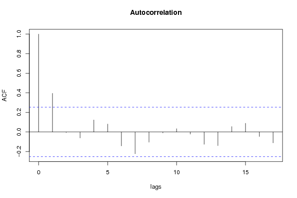
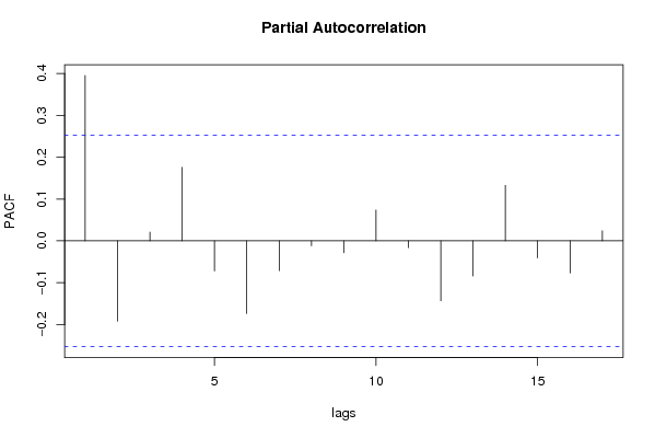
Title produced by software

(Partial) Autocorrelation Function

Date of computation

Mon, 08 Dec 2008 09:32:34 -0700

Cite this page as follows

Statistical Computations at FreeStatistics.org, Office for Research Development and Education, URL https://freestatistics.org/blog/index.php?v=date/2008/Dec/08/t122875423731tqsh3bimawh1b.htm/, Retrieved Thu, 16 May 2024 07:34:11 +0000

Statistical Computations at FreeStatistics.org, Office for Research Development and Education, URL https://freestatistics.org/blog/index.php?pk=30571, Retrieved Thu, 16 May 2024 07:34:11 +0000

QR Codes:

Paste this QR Code to cite your computation.

Original text written by user:

IsPrivate?

No (this computation is public)

User-defined keywords

Estimated Impact

167

Family? (F = Feedback message, R = changed R code, M = changed R Module, P = changed Parameters, D = changed Data)

F       [(Partial) Autocorrelation Function] [acf] [2008-12-08 16:32:34] [96839c4b6d4e03ef3851369c676780bf] [Current]

Feedback Forum

2008-12-15 13:32:31 [Bert Moons] [reply] 
correcte werkwijze en conclusie

Post a new message

Dataseries X:

Download CSV

Histogram

Boxplots

Summary of computational transaction
Raw Input	view raw input (R code)
Raw Output	view raw output of R engine
Computing time	2 seconds
R Server	'Herman Ole Andreas Wold' @ 193.190.124.10:1001

\begin{tabular}{lllllllll}
\hline
Summary of computational transaction \tabularnewline
Raw Input & view raw input (R code)  \tabularnewline
Raw Output & view raw output of R engine  \tabularnewline
Computing time & 2 seconds \tabularnewline
R Server & 'Herman Ole Andreas Wold' @ 193.190.124.10:1001 \tabularnewline
\hline
\end{tabular}
%Source: https://freestatistics.org/blog/index.php?pk=30571&T=0

[TABLE]
[ROW][C]Summary of computational transaction[/C][/ROW]
[ROW][C]Raw Input[/C][C]view raw input (R code) [/C][/ROW]
[ROW][C]Raw Output[/C][C]view raw output of R engine [/C][/ROW]
[ROW][C]Computing time[/C][C]2 seconds[/C][/ROW]
[ROW][C]R Server[/C][C]'Herman Ole Andreas Wold' @ 193.190.124.10:1001[/C][/ROW]
[/TABLE]
Source: https://freestatistics.org/blog/index.php?pk=30571&T=0

Globally Unique Identifier (entire table): ba.freestatistics.org/blog/index.php?pk=30571&T=0

As an alternative you can also use a QR Code:

The GUIDs for individual cells are displayed in the table below:

Summary of computational transaction
Raw Input	view raw input (R code)
Raw Output	view raw output of R engine
Computing time	2 seconds
R Server	'Herman Ole Andreas Wold' @ 193.190.124.10:1001

Autocorrelation Function
Time lag k	ACF(k)	T-STAT	P-value
1	0.395218	3.0613	0.001647
2	-0.00565	-0.0438	0.482617
3	-0.061508	-0.4764	0.317745
4	0.122969	0.9525	0.17233
5	0.0813	0.6297	0.265625
6	-0.142807	-1.1062	0.136532
7	-0.222917	-1.7267	0.044683
8	-0.104309	-0.808	0.211148
9	-0.009564	-0.0741	0.470594
10	0.033964	0.2631	0.396693
11	-0.021901	-0.1696	0.432931
12	-0.126027	-0.9762	0.166442
13	-0.139277	-1.0788	0.14249
14	0.055589	0.4306	0.334155
15	0.088793	0.6878	0.247118
16	-0.046602	-0.361	0.359692
17	-0.111319	-0.8623	0.195985

\begin{tabular}{lllllllll}
\hline
Autocorrelation Function \tabularnewline
Time lag k & ACF(k) & T-STAT & P-value \tabularnewline
1 & 0.395218 & 3.0613 & 0.001647 \tabularnewline
2 & -0.00565 & -0.0438 & 0.482617 \tabularnewline
3 & -0.061508 & -0.4764 & 0.317745 \tabularnewline
4 & 0.122969 & 0.9525 & 0.17233 \tabularnewline
5 & 0.0813 & 0.6297 & 0.265625 \tabularnewline
6 & -0.142807 & -1.1062 & 0.136532 \tabularnewline
7 & -0.222917 & -1.7267 & 0.044683 \tabularnewline
8 & -0.104309 & -0.808 & 0.211148 \tabularnewline
9 & -0.009564 & -0.0741 & 0.470594 \tabularnewline
10 & 0.033964 & 0.2631 & 0.396693 \tabularnewline
11 & -0.021901 & -0.1696 & 0.432931 \tabularnewline
12 & -0.126027 & -0.9762 & 0.166442 \tabularnewline
13 & -0.139277 & -1.0788 & 0.14249 \tabularnewline
14 & 0.055589 & 0.4306 & 0.334155 \tabularnewline
15 & 0.088793 & 0.6878 & 0.247118 \tabularnewline
16 & -0.046602 & -0.361 & 0.359692 \tabularnewline
17 & -0.111319 & -0.8623 & 0.195985 \tabularnewline
\hline
\end{tabular}
%Source: https://freestatistics.org/blog/index.php?pk=30571&T=1

[TABLE]
[ROW][C]Autocorrelation Function[/C][/ROW]
[ROW][C]Time lag k[/C][C]ACF(k)[/C][C]T-STAT[/C][C]P-value[/C][/ROW]
[ROW][C]1[/C][C]0.395218[/C][C]3.0613[/C][C]0.001647[/C][/ROW]
[ROW][C]2[/C][C]-0.00565[/C][C]-0.0438[/C][C]0.482617[/C][/ROW]
[ROW][C]3[/C][C]-0.061508[/C][C]-0.4764[/C][C]0.317745[/C][/ROW]
[ROW][C]4[/C][C]0.122969[/C][C]0.9525[/C][C]0.17233[/C][/ROW]
[ROW][C]5[/C][C]0.0813[/C][C]0.6297[/C][C]0.265625[/C][/ROW]
[ROW][C]6[/C][C]-0.142807[/C][C]-1.1062[/C][C]0.136532[/C][/ROW]
[ROW][C]7[/C][C]-0.222917[/C][C]-1.7267[/C][C]0.044683[/C][/ROW]
[ROW][C]8[/C][C]-0.104309[/C][C]-0.808[/C][C]0.211148[/C][/ROW]
[ROW][C]9[/C][C]-0.009564[/C][C]-0.0741[/C][C]0.470594[/C][/ROW]
[ROW][C]10[/C][C]0.033964[/C][C]0.2631[/C][C]0.396693[/C][/ROW]
[ROW][C]11[/C][C]-0.021901[/C][C]-0.1696[/C][C]0.432931[/C][/ROW]
[ROW][C]12[/C][C]-0.126027[/C][C]-0.9762[/C][C]0.166442[/C][/ROW]
[ROW][C]13[/C][C]-0.139277[/C][C]-1.0788[/C][C]0.14249[/C][/ROW]
[ROW][C]14[/C][C]0.055589[/C][C]0.4306[/C][C]0.334155[/C][/ROW]
[ROW][C]15[/C][C]0.088793[/C][C]0.6878[/C][C]0.247118[/C][/ROW]
[ROW][C]16[/C][C]-0.046602[/C][C]-0.361[/C][C]0.359692[/C][/ROW]
[ROW][C]17[/C][C]-0.111319[/C][C]-0.8623[/C][C]0.195985[/C][/ROW]
[/TABLE]
Source: https://freestatistics.org/blog/index.php?pk=30571&T=1

Globally Unique Identifier (entire table): ba.freestatistics.org/blog/index.php?pk=30571&T=1

As an alternative you can also use a QR Code:

The GUIDs for individual cells are displayed in the table below:

Autocorrelation Function
Time lag k	ACF(k)	T-STAT	P-value
1	0.395218	3.0613	0.001647
2	-0.00565	-0.0438	0.482617
3	-0.061508	-0.4764	0.317745
4	0.122969	0.9525	0.17233
5	0.0813	0.6297	0.265625
6	-0.142807	-1.1062	0.136532
7	-0.222917	-1.7267	0.044683
8	-0.104309	-0.808	0.211148
9	-0.009564	-0.0741	0.470594
10	0.033964	0.2631	0.396693
11	-0.021901	-0.1696	0.432931
12	-0.126027	-0.9762	0.166442
13	-0.139277	-1.0788	0.14249
14	0.055589	0.4306	0.334155
15	0.088793	0.6878	0.247118
16	-0.046602	-0.361	0.359692
17	-0.111319	-0.8623	0.195985

Partial Autocorrelation Function
Time lag k	PACF(k)	T-STAT	P-value
1	0.395218	3.0613	0.001647
2	-0.191807	-1.4857	0.071293
3	0.020865	0.1616	0.436073
4	0.175776	1.3616	0.089215
5	-0.072028	-0.5579	0.289487
6	-0.173775	-1.3461	0.091675
7	-0.071196	-0.5515	0.291677
8	-0.011657	-0.0903	0.464178
9	-0.028474	-0.2206	0.413091
10	0.073848	0.572	0.284723
11	-0.016348	-0.1266	0.449827
12	-0.143265	-1.1097	0.135773
13	-0.084036	-0.6509	0.258786
14	0.13271	1.028	0.154046
15	-0.040896	-0.3168	0.376257
16	-0.076858	-0.5953	0.276927
17	0.024004	0.1859	0.42656

\begin{tabular}{lllllllll}
\hline
Partial Autocorrelation Function \tabularnewline
Time lag k & PACF(k) & T-STAT & P-value \tabularnewline
1 & 0.395218 & 3.0613 & 0.001647 \tabularnewline
2 & -0.191807 & -1.4857 & 0.071293 \tabularnewline
3 & 0.020865 & 0.1616 & 0.436073 \tabularnewline
4 & 0.175776 & 1.3616 & 0.089215 \tabularnewline
5 & -0.072028 & -0.5579 & 0.289487 \tabularnewline
6 & -0.173775 & -1.3461 & 0.091675 \tabularnewline
7 & -0.071196 & -0.5515 & 0.291677 \tabularnewline
8 & -0.011657 & -0.0903 & 0.464178 \tabularnewline
9 & -0.028474 & -0.2206 & 0.413091 \tabularnewline
10 & 0.073848 & 0.572 & 0.284723 \tabularnewline
11 & -0.016348 & -0.1266 & 0.449827 \tabularnewline
12 & -0.143265 & -1.1097 & 0.135773 \tabularnewline
13 & -0.084036 & -0.6509 & 0.258786 \tabularnewline
14 & 0.13271 & 1.028 & 0.154046 \tabularnewline
15 & -0.040896 & -0.3168 & 0.376257 \tabularnewline
16 & -0.076858 & -0.5953 & 0.276927 \tabularnewline
17 & 0.024004 & 0.1859 & 0.42656 \tabularnewline
\hline
\end{tabular}
%Source: https://freestatistics.org/blog/index.php?pk=30571&T=2

[TABLE]
[ROW][C]Partial Autocorrelation Function[/C][/ROW]
[ROW][C]Time lag k[/C][C]PACF(k)[/C][C]T-STAT[/C][C]P-value[/C][/ROW]
[ROW][C]1[/C][C]0.395218[/C][C]3.0613[/C][C]0.001647[/C][/ROW]
[ROW][C]2[/C][C]-0.191807[/C][C]-1.4857[/C][C]0.071293[/C][/ROW]
[ROW][C]3[/C][C]0.020865[/C][C]0.1616[/C][C]0.436073[/C][/ROW]
[ROW][C]4[/C][C]0.175776[/C][C]1.3616[/C][C]0.089215[/C][/ROW]
[ROW][C]5[/C][C]-0.072028[/C][C]-0.5579[/C][C]0.289487[/C][/ROW]
[ROW][C]6[/C][C]-0.173775[/C][C]-1.3461[/C][C]0.091675[/C][/ROW]
[ROW][C]7[/C][C]-0.071196[/C][C]-0.5515[/C][C]0.291677[/C][/ROW]
[ROW][C]8[/C][C]-0.011657[/C][C]-0.0903[/C][C]0.464178[/C][/ROW]
[ROW][C]9[/C][C]-0.028474[/C][C]-0.2206[/C][C]0.413091[/C][/ROW]
[ROW][C]10[/C][C]0.073848[/C][C]0.572[/C][C]0.284723[/C][/ROW]
[ROW][C]11[/C][C]-0.016348[/C][C]-0.1266[/C][C]0.449827[/C][/ROW]
[ROW][C]12[/C][C]-0.143265[/C][C]-1.1097[/C][C]0.135773[/C][/ROW]
[ROW][C]13[/C][C]-0.084036[/C][C]-0.6509[/C][C]0.258786[/C][/ROW]
[ROW][C]14[/C][C]0.13271[/C][C]1.028[/C][C]0.154046[/C][/ROW]
[ROW][C]15[/C][C]-0.040896[/C][C]-0.3168[/C][C]0.376257[/C][/ROW]
[ROW][C]16[/C][C]-0.076858[/C][C]-0.5953[/C][C]0.276927[/C][/ROW]
[ROW][C]17[/C][C]0.024004[/C][C]0.1859[/C][C]0.42656[/C][/ROW]
[/TABLE]
Source: https://freestatistics.org/blog/index.php?pk=30571&T=2

Globally Unique Identifier (entire table): ba.freestatistics.org/blog/index.php?pk=30571&T=2

As an alternative you can also use a QR Code:

The GUIDs for individual cells are displayed in the table below:

Partial Autocorrelation Function
Time lag k	PACF(k)	T-STAT	P-value
1	0.395218	3.0613	0.001647
2	-0.191807	-1.4857	0.071293
3	0.020865	0.1616	0.436073
4	0.175776	1.3616	0.089215
5	-0.072028	-0.5579	0.289487
6	-0.173775	-1.3461	0.091675
7	-0.071196	-0.5515	0.291677
8	-0.011657	-0.0903	0.464178
9	-0.028474	-0.2206	0.413091
10	0.073848	0.572	0.284723
11	-0.016348	-0.1266	0.449827
12	-0.143265	-1.1097	0.135773
13	-0.084036	-0.6509	0.258786
14	0.13271	1.028	0.154046
15	-0.040896	-0.3168	0.376257
16	-0.076858	-0.5953	0.276927
17	0.024004	0.1859	0.42656

Figure 1

PNG link

Postscript link

PDF link

Figure 2

PNG link

Postscript link

PDF link

Parameters (Session):

par1 = Default ; par2 = -2.0 ; par3 = 1 ; par4 = 0 ; par5 = 12 ;

Parameters (R input):

par1 = Default ; par2 = -2.0 ; par3 = 1 ; par4 = 0 ; par5 = 12 ;

R code (references can be found in the software module):

if (par1 == 'Default') {
par1 = 10*log10(length(x))
} else {
par1 <- as.numeric(par1)
}
par2 <- as.numeric(par2)
par3 <- as.numeric(par3)
par4 <- as.numeric(par4)
par5 <- as.numeric(par5)
if (par2 == 0) {
x <- log(x)
} else {
x <- (x ^ par2 - 1) / par2
}
if (par3 > 0) x <- diff(x,lag=1,difference=par3)
if (par4 > 0) x <- diff(x,lag=par5,difference=par4)
bitmap(file='pic1.png')
racf <- acf(x,par1,main='Autocorrelation',xlab='lags',ylab='ACF')
dev.off()
bitmap(file='pic2.png')
rpacf <- pacf(x,par1,main='Partial Autocorrelation',xlab='lags',ylab='PACF')
dev.off()
(myacf <- c(racf$acf))
(mypacf <- c(rpacf$acf))
lengthx <- length(x)
sqrtn <- sqrt(lengthx)
load(file='createtable')
a<-table.start()
a<-table.row.start(a)
a<-table.element(a,'Autocorrelation Function',4,TRUE)
a<-table.row.end(a)
a<-table.row.start(a)
a<-table.element(a,'Time lag k',header=TRUE)
a<-table.element(a,hyperlink('basics.htm','ACF(k)','click here for more information about the Autocorrelation Function'),header=TRUE)
a<-table.element(a,'T-STAT',header=TRUE)
a<-table.element(a,'P-value',header=TRUE)
a<-table.row.end(a)
for (i in 2:(par1+1)) {
a<-table.row.start(a)
a<-table.element(a,i-1,header=TRUE)
a<-table.element(a,round(myacf[i],6))
mytstat <- myacf[i]*sqrtn
a<-table.element(a,round(mytstat,4))
a<-table.element(a,round(1-pt(abs(mytstat),lengthx),6))
a<-table.row.end(a)
}
a<-table.end(a)
table.save(a,file='mytable.tab')
a<-table.start()
a<-table.row.start(a)
a<-table.element(a,'Partial Autocorrelation Function',4,TRUE)
a<-table.row.end(a)
a<-table.row.start(a)
a<-table.element(a,'Time lag k',header=TRUE)
a<-table.element(a,hyperlink('basics.htm','PACF(k)','click here for more information about the Partial Autocorrelation Function'),header=TRUE)
a<-table.element(a,'T-STAT',header=TRUE)
a<-table.element(a,'P-value',header=TRUE)
a<-table.row.end(a)
for (i in 1:par1) {
a<-table.row.start(a)
a<-table.element(a,i,header=TRUE)
a<-table.element(a,round(mypacf[i],6))
mytstat <- mypacf[i]*sqrtn
a<-table.element(a,round(mytstat,4))
a<-table.element(a,round(1-pt(abs(mytstat),lengthx),6))
a<-table.row.end(a)
}
a<-table.end(a)
table.save(a,file='mytable1.tab')

Free Statistics

Description of Statistical Computation

Tree of Dependent Computations

Dataset

Tables (Output of Computation)

Figures (Output of Computation)

Input Parameters & R Code