Repository of Reproducible Computations

Free Statistics

of Irreproducible Research!

Author's title

Author

*The author of this computation has been verified*

R Software Module

rwasp_autocorrelation.wasp

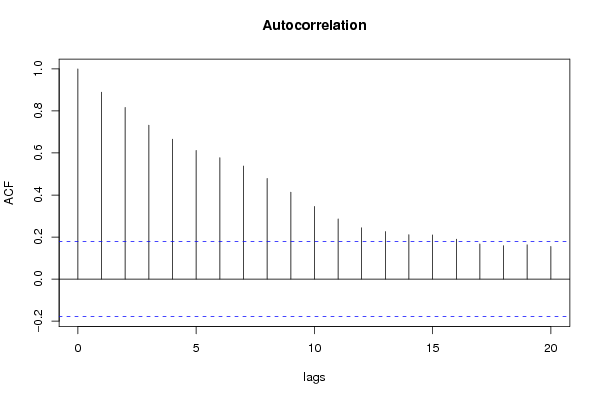
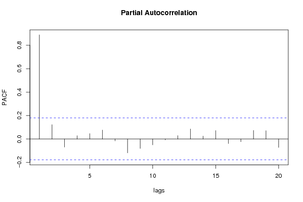
Title produced by software

(Partial) Autocorrelation Function

Date of computation

Sun, 07 Dec 2008 06:20:49 -0700

Cite this page as follows

Statistical Computations at FreeStatistics.org, Office for Research Development and Education, URL https://freestatistics.org/blog/index.php?v=date/2008/Dec/07/t12286561034vxisomspi42eh4.htm/, Retrieved Wed, 22 May 2024 12:37:25 +0000

Statistical Computations at FreeStatistics.org, Office for Research Development and Education, URL https://freestatistics.org/blog/index.php?pk=29949, Retrieved Wed, 22 May 2024 12:37:25 +0000

QR Codes:

Paste this QR Code to cite your computation.

Original text written by user:

IsPrivate?

No (this computation is public)

User-defined keywords

Estimated Impact

256

Family? (F = Feedback message, R = changed R code, M = changed R Module, P = changed Parameters, D = changed Data)

F     [Univariate Data Series] [Airline data] [2007-10-18 09:58:47] [42daae401fd3def69a25014f2252b4c2]
F RMPD  [Variance Reduction Matrix] [] [2008-11-30 18:13:06] [b745fd448f60064800b631a75a630267]
F RM D    [Standard Deviation-Mean Plot] [SMP Q1] [2008-12-07 13:12:10] [e5d91604aae608e98a8ea24759233f66]
F RM        [Variance Reduction Matrix] [VRM Q1] [2008-12-07 13:13:31] [e5d91604aae608e98a8ea24759233f66]
F RMP           [(Partial) Autocorrelation Function] [ACF Q2] [2008-12-07 13:20:49] [55ca0ca4a201c9689dcf5fae352c92eb] [Current]
- RMP             [Spectral Analysis] [Spectral Q2] [2008-12-07 13:23:21] [e5d91604aae608e98a8ea24759233f66] 
F   P               [Spectral Analysis] [Spectral Q3] [2008-12-07 13:28:29] [e5d91604aae608e98a8ea24759233f66] 
-   P                 [Spectral Analysis] [spectrum aangepast] [2008-12-18 14:46:11] [e5d91604aae608e98a8ea24759233f66] 
-                   [Spectral Analysis] [spectrum] [2008-12-18 14:39:41] [e5d91604aae608e98a8ea24759233f66] 
-    D                [Spectral Analysis] [spectrum zonder d...] [2008-12-18 15:10:35] [e5d91604aae608e98a8ea24759233f66] 
-    D                  [Spectral Analysis] [spectrum aangepast] [2008-12-18 15:14:31] [e5d91604aae608e98a8ea24759233f66] 
F   P             [(Partial) Autocorrelation Function] [ACF Q3] [2008-12-07 13:30:19] [e5d91604aae608e98a8ea24759233f66] 
F RMP             [ARIMA Backward Selection] [ARMA Q5] [2008-12-07 13:46:58] [e5d91604aae608e98a8ea24759233f66] 
-   P               [ARIMA Backward Selection] [ARIMA] [2008-12-10 17:52:14] [e5d91604aae608e98a8ea24759233f66] 
- RMPD              [Histogram] [Histogram inflatie] [2008-12-10 18:06:14] [e5d91604aae608e98a8ea24759233f66] 
- RMPD              [Variance Reduction Matrix] [VRM werkloosheid] [2008-12-10 18:11:05] [e5d91604aae608e98a8ea24759233f66] 
- RMPD              [Standard Deviation-Mean Plot] [SD mean plot] [2008-12-10 18:14:21] [e5d91604aae608e98a8ea24759233f66] 
-   PD              [ARIMA Backward Selection] [ARIMA Inflatie op...] [2008-12-10 18:24:04] [e5d91604aae608e98a8ea24759233f66] 
-   PD              [ARIMA Backward Selection] [ARIMA Inflatie op...] [2008-12-10 18:32:43] [e5d91604aae608e98a8ea24759233f66] 
-   P                 [ARIMA Backward Selection] [Arima backward 1] [2008-12-18 15:19:24] [e5d91604aae608e98a8ea24759233f66] 
F RMPD              [ARIMA Forecasting] [Forecasting Infla...] [2008-12-10 18:36:07] [e5d91604aae608e98a8ea24759233f66] 
-   P                 [ARIMA Forecasting] [Forecasting] [2008-12-18 16:01:41] [e5d91604aae608e98a8ea24759233f66] 
-   P             [(Partial) Autocorrelation Function] [Verbetering works...] [2008-12-15 09:55:17] [cf9c64468d04c2c4dd548cc66b4e3677] 

Feedback Forum

2008-12-15 09:59:25 [Jan Van Riet] [reply] 
Ik ga ermee akkoord dat je d op 1 instelt om de lange termijntrend eruit te halen, maar hierna ga je niet na of je nog seinzonaal gaat moeten differentiëren of niet (D=1). Dit blijkt niet het geval te zijn: 
 
http://www.freestatistics.org/blog/index.php?v=date/2008/Dec/15/t12293349817rgbdoqz25fddmj.htm 
 
(ik heb ook ineens de time lags op 36 gezet, zodat seizonaliteit zichtbaarder zou worden). 
 
Er is hier dus geen sprake van seizonaliteit.
2008-12-15 10:05:38 [Jan Van Riet] [reply] 
Ik zie dat je in je antwoord op vraag 4 dit wel gedaan hebt. Deze opmerking van mij is dus onterecht. 
  2008-12-15 10:07:34 [Jan Van Riet] [reply] 
correctie: vraag 3 bedoel ik.
2008-12-15 20:10:51 [Jeroen Aerts] [reply] 
Correcte berekening en goede commentaar.

Post a new message

Dataseries X:

Download CSV

Histogram

Boxplots

Summary of computational transaction
Raw Input	view raw input (R code)
Raw Output	view raw output of R engine
Computing time	1 seconds
R Server	'Sir Ronald Aylmer Fisher' @ 193.190.124.24

\begin{tabular}{lllllllll}
\hline
Summary of computational transaction \tabularnewline
Raw Input & view raw input (R code)  \tabularnewline
Raw Output & view raw output of R engine  \tabularnewline
Computing time & 1 seconds \tabularnewline
R Server & 'Sir Ronald Aylmer Fisher' @ 193.190.124.24 \tabularnewline
\hline
\end{tabular}
%Source: https://freestatistics.org/blog/index.php?pk=29949&T=0

[TABLE]
[ROW][C]Summary of computational transaction[/C][/ROW]
[ROW][C]Raw Input[/C][C]view raw input (R code) [/C][/ROW]
[ROW][C]Raw Output[/C][C]view raw output of R engine [/C][/ROW]
[ROW][C]Computing time[/C][C]1 seconds[/C][/ROW]
[ROW][C]R Server[/C][C]'Sir Ronald Aylmer Fisher' @ 193.190.124.24[/C][/ROW]
[/TABLE]
Source: https://freestatistics.org/blog/index.php?pk=29949&T=0

Globally Unique Identifier (entire table): ba.freestatistics.org/blog/index.php?pk=29949&T=0

As an alternative you can also use a QR Code:

The GUIDs for individual cells are displayed in the table below:

Summary of computational transaction
Raw Input	view raw input (R code)
Raw Output	view raw output of R engine
Computing time	1 seconds
R Server	'Sir Ronald Aylmer Fisher' @ 193.190.124.24

Autocorrelation Function
Time lag k	ACF(k)	T-STAT	P-value
1	0.889506	9.7441	0
2	0.816718	8.9467	0
3	0.732077	8.0195	0
4	0.665857	7.2941	0
5	0.611935	6.7034	0
6	0.577269	6.3237	0
7	0.537609	5.8892	0
8	0.478906	5.2462	0
9	0.413458	4.5292	7e-06
10	0.345303	3.7826	0.000122
11	0.286393	3.1373	0.001073
12	0.243622	2.6687	0.004333
13	0.225886	2.4745	0.007371
14	0.210896	2.3102	0.011291
15	0.209492	2.2949	0.011739
16	0.189793	2.0791	0.01987
17	0.167439	1.8342	0.034551
18	0.158464	1.7359	0.042575
19	0.162701	1.7823	0.038615
20	0.154857	1.6964	0.046204

\begin{tabular}{lllllllll}
\hline
Autocorrelation Function \tabularnewline
Time lag k & ACF(k) & T-STAT & P-value \tabularnewline
1 & 0.889506 & 9.7441 & 0 \tabularnewline
2 & 0.816718 & 8.9467 & 0 \tabularnewline
3 & 0.732077 & 8.0195 & 0 \tabularnewline
4 & 0.665857 & 7.2941 & 0 \tabularnewline
5 & 0.611935 & 6.7034 & 0 \tabularnewline
6 & 0.577269 & 6.3237 & 0 \tabularnewline
7 & 0.537609 & 5.8892 & 0 \tabularnewline
8 & 0.478906 & 5.2462 & 0 \tabularnewline
9 & 0.413458 & 4.5292 & 7e-06 \tabularnewline
10 & 0.345303 & 3.7826 & 0.000122 \tabularnewline
11 & 0.286393 & 3.1373 & 0.001073 \tabularnewline
12 & 0.243622 & 2.6687 & 0.004333 \tabularnewline
13 & 0.225886 & 2.4745 & 0.007371 \tabularnewline
14 & 0.210896 & 2.3102 & 0.011291 \tabularnewline
15 & 0.209492 & 2.2949 & 0.011739 \tabularnewline
16 & 0.189793 & 2.0791 & 0.01987 \tabularnewline
17 & 0.167439 & 1.8342 & 0.034551 \tabularnewline
18 & 0.158464 & 1.7359 & 0.042575 \tabularnewline
19 & 0.162701 & 1.7823 & 0.038615 \tabularnewline
20 & 0.154857 & 1.6964 & 0.046204 \tabularnewline
\hline
\end{tabular}
%Source: https://freestatistics.org/blog/index.php?pk=29949&T=1

[TABLE]
[ROW][C]Autocorrelation Function[/C][/ROW]
[ROW][C]Time lag k[/C][C]ACF(k)[/C][C]T-STAT[/C][C]P-value[/C][/ROW]
[ROW][C]1[/C][C]0.889506[/C][C]9.7441[/C][C]0[/C][/ROW]
[ROW][C]2[/C][C]0.816718[/C][C]8.9467[/C][C]0[/C][/ROW]
[ROW][C]3[/C][C]0.732077[/C][C]8.0195[/C][C]0[/C][/ROW]
[ROW][C]4[/C][C]0.665857[/C][C]7.2941[/C][C]0[/C][/ROW]
[ROW][C]5[/C][C]0.611935[/C][C]6.7034[/C][C]0[/C][/ROW]
[ROW][C]6[/C][C]0.577269[/C][C]6.3237[/C][C]0[/C][/ROW]
[ROW][C]7[/C][C]0.537609[/C][C]5.8892[/C][C]0[/C][/ROW]
[ROW][C]8[/C][C]0.478906[/C][C]5.2462[/C][C]0[/C][/ROW]
[ROW][C]9[/C][C]0.413458[/C][C]4.5292[/C][C]7e-06[/C][/ROW]
[ROW][C]10[/C][C]0.345303[/C][C]3.7826[/C][C]0.000122[/C][/ROW]
[ROW][C]11[/C][C]0.286393[/C][C]3.1373[/C][C]0.001073[/C][/ROW]
[ROW][C]12[/C][C]0.243622[/C][C]2.6687[/C][C]0.004333[/C][/ROW]
[ROW][C]13[/C][C]0.225886[/C][C]2.4745[/C][C]0.007371[/C][/ROW]
[ROW][C]14[/C][C]0.210896[/C][C]2.3102[/C][C]0.011291[/C][/ROW]
[ROW][C]15[/C][C]0.209492[/C][C]2.2949[/C][C]0.011739[/C][/ROW]
[ROW][C]16[/C][C]0.189793[/C][C]2.0791[/C][C]0.01987[/C][/ROW]
[ROW][C]17[/C][C]0.167439[/C][C]1.8342[/C][C]0.034551[/C][/ROW]
[ROW][C]18[/C][C]0.158464[/C][C]1.7359[/C][C]0.042575[/C][/ROW]
[ROW][C]19[/C][C]0.162701[/C][C]1.7823[/C][C]0.038615[/C][/ROW]
[ROW][C]20[/C][C]0.154857[/C][C]1.6964[/C][C]0.046204[/C][/ROW]
[/TABLE]
Source: https://freestatistics.org/blog/index.php?pk=29949&T=1

Globally Unique Identifier (entire table): ba.freestatistics.org/blog/index.php?pk=29949&T=1

As an alternative you can also use a QR Code:

The GUIDs for individual cells are displayed in the table below:

Autocorrelation Function
Time lag k	ACF(k)	T-STAT	P-value
1	0.889506	9.7441	0
2	0.816718	8.9467	0
3	0.732077	8.0195	0
4	0.665857	7.2941	0
5	0.611935	6.7034	0
6	0.577269	6.3237	0
7	0.537609	5.8892	0
8	0.478906	5.2462	0
9	0.413458	4.5292	7e-06
10	0.345303	3.7826	0.000122
11	0.286393	3.1373	0.001073
12	0.243622	2.6687	0.004333
13	0.225886	2.4745	0.007371
14	0.210896	2.3102	0.011291
15	0.209492	2.2949	0.011739
16	0.189793	2.0791	0.01987
17	0.167439	1.8342	0.034551
18	0.158464	1.7359	0.042575
19	0.162701	1.7823	0.038615
20	0.154857	1.6964	0.046204

Partial Autocorrelation Function
Time lag k	PACF(k)	T-STAT	P-value
1	0.889506	9.7441	0
2	0.122125	1.3378	0.091745
3	-0.069572	-0.7621	0.22374
4	0.028088	0.3077	0.379426
5	0.04607	0.5047	0.307357
6	0.07653	0.8383	0.201753
7	-0.016843	-0.1845	0.426962
8	-0.119194	-1.3057	0.097075
9	-0.081234	-0.8899	0.187657
10	-0.050593	-0.5542	0.290229
11	-0.007741	-0.0848	0.466281
12	0.028975	0.3174	0.375743
13	0.085524	0.9369	0.175355
14	0.024426	0.2676	0.394743
15	0.072282	0.7918	0.215017
16	-0.039213	-0.4296	0.334145
17	-0.023678	-0.2594	0.397895
18	0.073514	0.8053	0.211118
19	0.070583	0.7732	0.220464
20	-0.073005	-0.7997	0.212723

\begin{tabular}{lllllllll}
\hline
Partial Autocorrelation Function \tabularnewline
Time lag k & PACF(k) & T-STAT & P-value \tabularnewline
1 & 0.889506 & 9.7441 & 0 \tabularnewline
2 & 0.122125 & 1.3378 & 0.091745 \tabularnewline
3 & -0.069572 & -0.7621 & 0.22374 \tabularnewline
4 & 0.028088 & 0.3077 & 0.379426 \tabularnewline
5 & 0.04607 & 0.5047 & 0.307357 \tabularnewline
6 & 0.07653 & 0.8383 & 0.201753 \tabularnewline
7 & -0.016843 & -0.1845 & 0.426962 \tabularnewline
8 & -0.119194 & -1.3057 & 0.097075 \tabularnewline
9 & -0.081234 & -0.8899 & 0.187657 \tabularnewline
10 & -0.050593 & -0.5542 & 0.290229 \tabularnewline
11 & -0.007741 & -0.0848 & 0.466281 \tabularnewline
12 & 0.028975 & 0.3174 & 0.375743 \tabularnewline
13 & 0.085524 & 0.9369 & 0.175355 \tabularnewline
14 & 0.024426 & 0.2676 & 0.394743 \tabularnewline
15 & 0.072282 & 0.7918 & 0.215017 \tabularnewline
16 & -0.039213 & -0.4296 & 0.334145 \tabularnewline
17 & -0.023678 & -0.2594 & 0.397895 \tabularnewline
18 & 0.073514 & 0.8053 & 0.211118 \tabularnewline
19 & 0.070583 & 0.7732 & 0.220464 \tabularnewline
20 & -0.073005 & -0.7997 & 0.212723 \tabularnewline
\hline
\end{tabular}
%Source: https://freestatistics.org/blog/index.php?pk=29949&T=2

[TABLE]
[ROW][C]Partial Autocorrelation Function[/C][/ROW]
[ROW][C]Time lag k[/C][C]PACF(k)[/C][C]T-STAT[/C][C]P-value[/C][/ROW]
[ROW][C]1[/C][C]0.889506[/C][C]9.7441[/C][C]0[/C][/ROW]
[ROW][C]2[/C][C]0.122125[/C][C]1.3378[/C][C]0.091745[/C][/ROW]
[ROW][C]3[/C][C]-0.069572[/C][C]-0.7621[/C][C]0.22374[/C][/ROW]
[ROW][C]4[/C][C]0.028088[/C][C]0.3077[/C][C]0.379426[/C][/ROW]
[ROW][C]5[/C][C]0.04607[/C][C]0.5047[/C][C]0.307357[/C][/ROW]
[ROW][C]6[/C][C]0.07653[/C][C]0.8383[/C][C]0.201753[/C][/ROW]
[ROW][C]7[/C][C]-0.016843[/C][C]-0.1845[/C][C]0.426962[/C][/ROW]
[ROW][C]8[/C][C]-0.119194[/C][C]-1.3057[/C][C]0.097075[/C][/ROW]
[ROW][C]9[/C][C]-0.081234[/C][C]-0.8899[/C][C]0.187657[/C][/ROW]
[ROW][C]10[/C][C]-0.050593[/C][C]-0.5542[/C][C]0.290229[/C][/ROW]
[ROW][C]11[/C][C]-0.007741[/C][C]-0.0848[/C][C]0.466281[/C][/ROW]
[ROW][C]12[/C][C]0.028975[/C][C]0.3174[/C][C]0.375743[/C][/ROW]
[ROW][C]13[/C][C]0.085524[/C][C]0.9369[/C][C]0.175355[/C][/ROW]
[ROW][C]14[/C][C]0.024426[/C][C]0.2676[/C][C]0.394743[/C][/ROW]
[ROW][C]15[/C][C]0.072282[/C][C]0.7918[/C][C]0.215017[/C][/ROW]
[ROW][C]16[/C][C]-0.039213[/C][C]-0.4296[/C][C]0.334145[/C][/ROW]
[ROW][C]17[/C][C]-0.023678[/C][C]-0.2594[/C][C]0.397895[/C][/ROW]
[ROW][C]18[/C][C]0.073514[/C][C]0.8053[/C][C]0.211118[/C][/ROW]
[ROW][C]19[/C][C]0.070583[/C][C]0.7732[/C][C]0.220464[/C][/ROW]
[ROW][C]20[/C][C]-0.073005[/C][C]-0.7997[/C][C]0.212723[/C][/ROW]
[/TABLE]
Source: https://freestatistics.org/blog/index.php?pk=29949&T=2

Globally Unique Identifier (entire table): ba.freestatistics.org/blog/index.php?pk=29949&T=2

As an alternative you can also use a QR Code:

The GUIDs for individual cells are displayed in the table below:

Partial Autocorrelation Function
Time lag k	PACF(k)	T-STAT	P-value
1	0.889506	9.7441	0
2	0.122125	1.3378	0.091745
3	-0.069572	-0.7621	0.22374
4	0.028088	0.3077	0.379426
5	0.04607	0.5047	0.307357
6	0.07653	0.8383	0.201753
7	-0.016843	-0.1845	0.426962
8	-0.119194	-1.3057	0.097075
9	-0.081234	-0.8899	0.187657
10	-0.050593	-0.5542	0.290229
11	-0.007741	-0.0848	0.466281
12	0.028975	0.3174	0.375743
13	0.085524	0.9369	0.175355
14	0.024426	0.2676	0.394743
15	0.072282	0.7918	0.215017
16	-0.039213	-0.4296	0.334145
17	-0.023678	-0.2594	0.397895
18	0.073514	0.8053	0.211118
19	0.070583	0.7732	0.220464
20	-0.073005	-0.7997	0.212723

Figure 1

PNG link

Postscript link

PDF link

Figure 2

PNG link

Postscript link

PDF link

Parameters (Session):

par1 = Default ; par2 = 1.3 ; par3 = 0 ; par4 = 0 ; par5 = 12 ;

Parameters (R input):

par1 = Default ; par2 = 1.3 ; par3 = 0 ; par4 = 0 ; par5 = 12 ;

R code (references can be found in the software module):

if (par1 == 'Default') {
par1 = 10*log10(length(x))
} else {
par1 <- as.numeric(par1)
}
par2 <- as.numeric(par2)
par3 <- as.numeric(par3)
par4 <- as.numeric(par4)
par5 <- as.numeric(par5)
if (par2 == 0) {
x <- log(x)
} else {
x <- (x ^ par2 - 1) / par2
}
if (par3 > 0) x <- diff(x,lag=1,difference=par3)
if (par4 > 0) x <- diff(x,lag=par5,difference=par4)
bitmap(file='pic1.png')
racf <- acf(x,par1,main='Autocorrelation',xlab='lags',ylab='ACF')
dev.off()
bitmap(file='pic2.png')
rpacf <- pacf(x,par1,main='Partial Autocorrelation',xlab='lags',ylab='PACF')
dev.off()
(myacf <- c(racf$acf))
(mypacf <- c(rpacf$acf))
lengthx <- length(x)
sqrtn <- sqrt(lengthx)
load(file='createtable')
a<-table.start()
a<-table.row.start(a)
a<-table.element(a,'Autocorrelation Function',4,TRUE)
a<-table.row.end(a)
a<-table.row.start(a)
a<-table.element(a,'Time lag k',header=TRUE)
a<-table.element(a,hyperlink('basics.htm','ACF(k)','click here for more information about the Autocorrelation Function'),header=TRUE)
a<-table.element(a,'T-STAT',header=TRUE)
a<-table.element(a,'P-value',header=TRUE)
a<-table.row.end(a)
for (i in 2:(par1+1)) {
a<-table.row.start(a)
a<-table.element(a,i-1,header=TRUE)
a<-table.element(a,round(myacf[i],6))
mytstat <- myacf[i]*sqrtn
a<-table.element(a,round(mytstat,4))
a<-table.element(a,round(1-pt(abs(mytstat),lengthx),6))
a<-table.row.end(a)
}
a<-table.end(a)
table.save(a,file='mytable.tab')
a<-table.start()
a<-table.row.start(a)
a<-table.element(a,'Partial Autocorrelation Function',4,TRUE)
a<-table.row.end(a)
a<-table.row.start(a)
a<-table.element(a,'Time lag k',header=TRUE)
a<-table.element(a,hyperlink('basics.htm','PACF(k)','click here for more information about the Partial Autocorrelation Function'),header=TRUE)
a<-table.element(a,'T-STAT',header=TRUE)
a<-table.element(a,'P-value',header=TRUE)
a<-table.row.end(a)
for (i in 1:par1) {
a<-table.row.start(a)
a<-table.element(a,i,header=TRUE)
a<-table.element(a,round(mypacf[i],6))
mytstat <- mypacf[i]*sqrtn
a<-table.element(a,round(mytstat,4))
a<-table.element(a,round(1-pt(abs(mytstat),lengthx),6))
a<-table.row.end(a)
}
a<-table.end(a)
table.save(a,file='mytable1.tab')

Free Statistics

Description of Statistical Computation

Tree of Dependent Computations

Dataset

Tables (Output of Computation)

Figures (Output of Computation)

Input Parameters & R Code