Free Statistics
of Irreproducible Research!
Description of Statistical Computation | |||||||||||||||||||||||||||||||||||||||||||||||||||||||||||||||||||||
|---|---|---|---|---|---|---|---|---|---|---|---|---|---|---|---|---|---|---|---|---|---|---|---|---|---|---|---|---|---|---|---|---|---|---|---|---|---|---|---|---|---|---|---|---|---|---|---|---|---|---|---|---|---|---|---|---|---|---|---|---|---|---|---|---|---|---|---|---|---|
| Author's title | |||||||||||||||||||||||||||||||||||||||||||||||||||||||||||||||||||||
| Author | *The author of this computation has been verified* | ||||||||||||||||||||||||||||||||||||||||||||||||||||||||||||||||||||
| R Software Module | rwasp_pairs.wasp | ||||||||||||||||||||||||||||||||||||||||||||||||||||||||||||||||||||
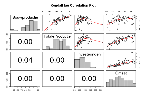
| Title produced by software | Kendall tau Correlation Matrix | ||||||||||||||||||||||||||||||||||||||||||||||||||||||||||||||||||||
| Date of computation | Fri, 05 Dec 2008 09:54:10 -0700 | ||||||||||||||||||||||||||||||||||||||||||||||||||||||||||||||||||||
| Cite this page as follows | Statistical Computations at FreeStatistics.org, Office for Research Development and Education, URL https://freestatistics.org/blog/index.php?v=date/2008/Dec/05/t1228496316impkdxr2hnn6ivf.htm/, Retrieved Thu, 16 May 2024 07:54:42 +0000 | ||||||||||||||||||||||||||||||||||||||||||||||||||||||||||||||||||||
| Statistical Computations at FreeStatistics.org, Office for Research Development and Education, URL https://freestatistics.org/blog/index.php?pk=29340, Retrieved Thu, 16 May 2024 07:54:42 +0000 | |||||||||||||||||||||||||||||||||||||||||||||||||||||||||||||||||||||
| QR Codes: | |||||||||||||||||||||||||||||||||||||||||||||||||||||||||||||||||||||
|
| |||||||||||||||||||||||||||||||||||||||||||||||||||||||||||||||||||||
| Original text written by user: | |||||||||||||||||||||||||||||||||||||||||||||||||||||||||||||||||||||
| IsPrivate? | No (this computation is public) | ||||||||||||||||||||||||||||||||||||||||||||||||||||||||||||||||||||
| User-defined keywords | |||||||||||||||||||||||||||||||||||||||||||||||||||||||||||||||||||||
| Estimated Impact | 178 | ||||||||||||||||||||||||||||||||||||||||||||||||||||||||||||||||||||
Tree of Dependent Computations | |||||||||||||||||||||||||||||||||||||||||||||||||||||||||||||||||||||
| Family? (F = Feedback message, R = changed R code, M = changed R Module, P = changed Parameters, D = changed Data) | |||||||||||||||||||||||||||||||||||||||||||||||||||||||||||||||||||||
| - [Back to Back Histogram] [Btb histogram bou...] [2008-12-05 16:20:27] [aa5573c1db401b164e448aef050955a1] - PD [Back to Back Histogram] [Btb histogram bou...] [2008-12-05 16:24:17] [aa5573c1db401b164e448aef050955a1] - RMPD [Kendall tau Correlation Matrix] [Kendall Tau bouwp...] [2008-12-05 16:54:10] [8a1195ff8db4df756ce44b463a631c76] [Current] | |||||||||||||||||||||||||||||||||||||||||||||||||||||||||||||||||||||
| Feedback Forum | |||||||||||||||||||||||||||||||||||||||||||||||||||||||||||||||||||||
Post a new message | |||||||||||||||||||||||||||||||||||||||||||||||||||||||||||||||||||||
Dataset | |||||||||||||||||||||||||||||||||||||||||||||||||||||||||||||||||||||
| Dataseries X: | |||||||||||||||||||||||||||||||||||||||||||||||||||||||||||||||||||||
82.7 97.4 74.8 89.3 88.9 97 93.1 87.5 105.9 105.4 103.9 106.7 100.8 102.7 83.9 102.5 94 98.1 77.7 109.2 105 104.5 141.5 123.7 58.5 87.4 58.9 83.1 87.6 89.9 75.3 97 113.1 109.8 108.4 119.1 112.5 111.7 91 125.1 89.6 98.6 84.6 113.6 74.5 96.9 179.8 122.4 82.7 95.1 85.6 92.8 90.1 97 76.4 97.2 109.4 112.7 109.7 115.6 96 102.9 99.1 111.3 89.2 97.4 86.7 114.6 109.1 111.4 111.4 137.5 49.1 87.4 78.4 83.7 92.9 96.8 76.7 106 107.7 114.1 114.2 123.4 103.5 110.3 99.7 126.5 91.1 103.9 94.2 120 79.8 101.6 173.5 141.6 71.9 94.6 83.1 90.5 82.9 95.9 88.9 96.5 90.1 104.7 132 113.5 100.7 102.8 122.1 120.1 90.7 98.1 105.1 123.9 108.8 113.9 133.7 144.4 44.1 80.9 63.6 90.8 93.6 95.7 112.7 114.2 107.4 113.2 120.5 138.1 96.5 105.9 112 135 93.6 108.8 126.2 131.3 76.5 102.3 209.2 144.6 76.7 99 91 101.7 84 100.7 116.7 108.7 103.3 115.5 137.6 135.3 88.5 100.7 108.1 124.3 99 109.9 136.6 138.3 105.9 114.6 152.3 158.2 44.7 85.4 114.3 93.5 94 100.5 120.7 124.8 107.1 114.8 131.8 154.4 104.8 116.5 129.4 152.8 102.5 112.9 187.5 148.9 77.7 102 189.5 170.3 85.2 106 109.2 124.8 91.3 105.3 158.1 134.4 106.5 118.8 176.2 154 92.4 106.1 125.5 147.9 97.5 109.3 155 168.1 107 117.2 170.3 175.7 51.1 92.5 99.4 116.7 98.6 104.2 139.2 140.8 102.2 112.5 169.6 164.2 114.3 122.4 136.1 173.8 99.4 113.3 168.2 167.8 72.5 100 318.6 166.6 92.3 110.7 154.1 135.1 99.4 112.8 161.4 158.1 85.9 109.8 183.4 151.8 109.4 117.3 167.2 168.7 97.6 109.1 205.3 166.9 | |||||||||||||||||||||||||||||||||||||||||||||||||||||||||||||||||||||
Tables (Output of Computation) | |||||||||||||||||||||||||||||||||||||||||||||||||||||||||||||||||||||
| |||||||||||||||||||||||||||||||||||||||||||||||||||||||||||||||||||||
Figures (Output of Computation) | |||||||||||||||||||||||||||||||||||||||||||||||||||||||||||||||||||||
Input Parameters & R Code | |||||||||||||||||||||||||||||||||||||||||||||||||||||||||||||||||||||
| Parameters (Session): | |||||||||||||||||||||||||||||||||||||||||||||||||||||||||||||||||||||
| Parameters (R input): | |||||||||||||||||||||||||||||||||||||||||||||||||||||||||||||||||||||
| R code (references can be found in the software module): | |||||||||||||||||||||||||||||||||||||||||||||||||||||||||||||||||||||
panel.tau <- function(x, y, digits=2, prefix='', cex.cor) | |||||||||||||||||||||||||||||||||||||||||||||||||||||||||||||||||||||