Free Statistics
of Irreproducible Research!
Description of Statistical Computation | |||||||||||||||||||||
|---|---|---|---|---|---|---|---|---|---|---|---|---|---|---|---|---|---|---|---|---|---|
| Author's title | |||||||||||||||||||||
| Author | *The author of this computation has been verified* | ||||||||||||||||||||
| R Software Module | rwasp_meanplot.wasp | ||||||||||||||||||||
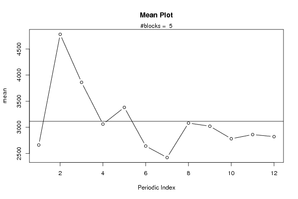
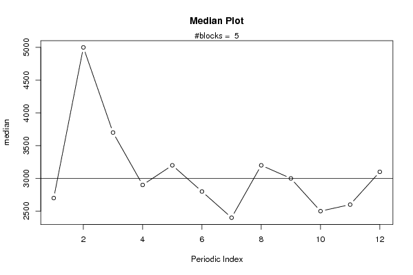
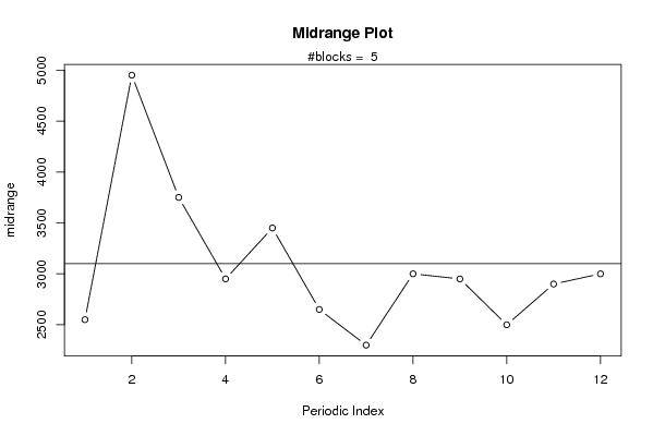
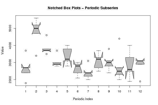
| Title produced by software | Mean Plot | ||||||||||||||||||||
| Date of computation | Fri, 05 Dec 2008 07:45:50 -0700 | ||||||||||||||||||||
| Cite this page as follows | Statistical Computations at FreeStatistics.org, Office for Research Development and Education, URL https://freestatistics.org/blog/index.php?v=date/2008/Dec/05/t1228488941rwkhmoja4kkh6hf.htm/, Retrieved Thu, 16 May 2024 06:21:11 +0000 | ||||||||||||||||||||
| Statistical Computations at FreeStatistics.org, Office for Research Development and Education, URL https://freestatistics.org/blog/index.php?pk=29293, Retrieved Thu, 16 May 2024 06:21:11 +0000 | |||||||||||||||||||||
| QR Codes: | |||||||||||||||||||||
|
| |||||||||||||||||||||
| Original text written by user: | st�phanie claes, kevin engels en katrien bourdiaudhy | ||||||||||||||||||||
| IsPrivate? | No (this computation is public) | ||||||||||||||||||||
| User-defined keywords | |||||||||||||||||||||
| Estimated Impact | 193 | ||||||||||||||||||||
Tree of Dependent Computations | |||||||||||||||||||||
| Family? (F = Feedback message, R = changed R code, M = changed R Module, P = changed Parameters, D = changed Data) | |||||||||||||||||||||
| F [Univariate Data Series] [blog 1e tijdreeks...] [2008-10-13 19:23:31] [7173087adebe3e3a714c80ea2417b3eb] - PD [Univariate Data Series] [tijdreeksen opnie...] [2008-10-19 17:18:46] [7173087adebe3e3a714c80ea2417b3eb] - RMP [Central Tendency] [tijdreeks 2 centr...] [2008-10-19 17:39:42] [7173087adebe3e3a714c80ea2417b3eb] - RMP [Mean Plot] [mean plot aanvrag...] [2008-12-05 14:45:50] [95d95b0e883740fcbc85e18ec42dcafb] [Current] | |||||||||||||||||||||
| Feedback Forum | |||||||||||||||||||||
Post a new message | |||||||||||||||||||||
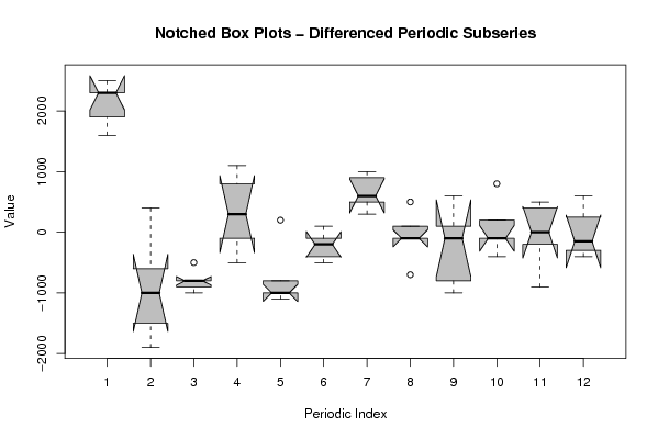
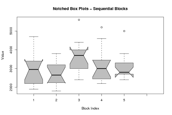
Dataset | |||||||||||||||||||||
| Dataseries X: | |||||||||||||||||||||
2400 4700 3700 2900 2800 3000 3100 3700 3000 2000 1900 1900 1800 3400 3800 2800 3100 2100 2000 2500 2400 2500 3300 3100 3700 5600 3700 2900 4000 2900 2400 3300 3800 4400 4000 3100 2700 5200 4600 3700 3200 2400 2200 3200 3100 2300 2500 2900 2700 5000 3500 3000 3800 2800 2400 2700 2800 2700 2600 3100 | |||||||||||||||||||||
Tables (Output of Computation) | |||||||||||||||||||||
| |||||||||||||||||||||
Figures (Output of Computation) | |||||||||||||||||||||
Input Parameters & R Code | |||||||||||||||||||||
| Parameters (Session): | |||||||||||||||||||||
| par1 = 12 ; | |||||||||||||||||||||
| Parameters (R input): | |||||||||||||||||||||
| par1 = 12 ; | |||||||||||||||||||||
| R code (references can be found in the software module): | |||||||||||||||||||||
par1 <- as.numeric(par1) | |||||||||||||||||||||