Free Statistics
of Irreproducible Research!
Description of Statistical Computation | |||||||||||||||||||||||||||||||||||||||||||||
|---|---|---|---|---|---|---|---|---|---|---|---|---|---|---|---|---|---|---|---|---|---|---|---|---|---|---|---|---|---|---|---|---|---|---|---|---|---|---|---|---|---|---|---|---|---|
| Author's title | |||||||||||||||||||||||||||||||||||||||||||||
| Author | *The author of this computation has been verified* | ||||||||||||||||||||||||||||||||||||||||||||
| R Software Module | rwasp_boxcoxlin.wasp | ||||||||||||||||||||||||||||||||||||||||||||
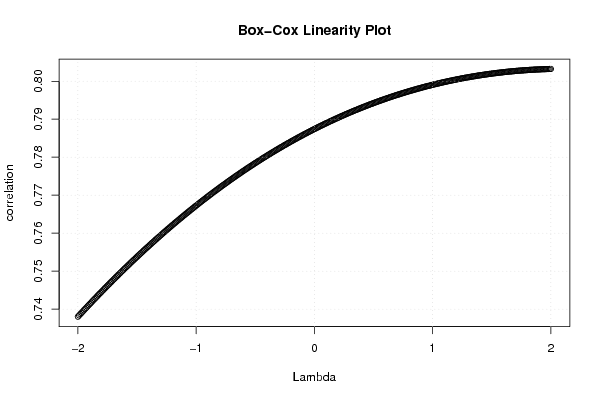
| Title produced by software | Box-Cox Linearity Plot | ||||||||||||||||||||||||||||||||||||||||||||
| Date of computation | Fri, 05 Dec 2008 07:29:26 -0700 | ||||||||||||||||||||||||||||||||||||||||||||
| Cite this page as follows | Statistical Computations at FreeStatistics.org, Office for Research Development and Education, URL https://freestatistics.org/blog/index.php?v=date/2008/Dec/05/t1228487418hoa8q7t48st8u2x.htm/, Retrieved Thu, 16 May 2024 11:09:08 +0000 | ||||||||||||||||||||||||||||||||||||||||||||
| Statistical Computations at FreeStatistics.org, Office for Research Development and Education, URL https://freestatistics.org/blog/index.php?pk=29278, Retrieved Thu, 16 May 2024 11:09:08 +0000 | |||||||||||||||||||||||||||||||||||||||||||||
| QR Codes: | |||||||||||||||||||||||||||||||||||||||||||||
|
| |||||||||||||||||||||||||||||||||||||||||||||
| Original text written by user: | |||||||||||||||||||||||||||||||||||||||||||||
| IsPrivate? | No (this computation is public) | ||||||||||||||||||||||||||||||||||||||||||||
| User-defined keywords | |||||||||||||||||||||||||||||||||||||||||||||
| Estimated Impact | 170 | ||||||||||||||||||||||||||||||||||||||||||||
Tree of Dependent Computations | |||||||||||||||||||||||||||||||||||||||||||||
| Family? (F = Feedback message, R = changed R code, M = changed R Module, P = changed Parameters, D = changed Data) | |||||||||||||||||||||||||||||||||||||||||||||
| - [Box-Cox Linearity Plot] [inv vs nt duurz cons] [2008-12-05 14:29:26] [fa8b44cd657c07c6ee11bb2476ca3f8d] [Current] | |||||||||||||||||||||||||||||||||||||||||||||
| Feedback Forum | |||||||||||||||||||||||||||||||||||||||||||||
Post a new message | |||||||||||||||||||||||||||||||||||||||||||||
Dataset | |||||||||||||||||||||||||||||||||||||||||||||
| Dataseries X: | |||||||||||||||||||||||||||||||||||||||||||||
93.0 99.2 112.2 112.1 103.3 108.2 90.4 72.8 111.0 117.9 111.3 110.5 94.8 100.4 132.1 114.6 101.9 130.2 84.0 86.4 122.3 120.9 110.2 112.6 102.0 105.0 130.5 115.5 103.7 130.9 89.1 93.8 123.8 111.9 118.3 116.9 103.6 116.6 141.3 107.0 125.2 136.4 91.6 95.3 132.3 130.6 131.9 118.6 114.3 111.3 126.5 112.1 119.3 142.4 101.1 97.4 129.1 136.9 129.8 123.9 | |||||||||||||||||||||||||||||||||||||||||||||
| Dataseries Y: | |||||||||||||||||||||||||||||||||||||||||||||
95,9 95,3 100,4 97,3 82,3 97,0 93,5 90,9 107,8 110,9 98,1 106,5 93,4 95,7 109,0 97,6 92,7 107,5 91,7 95,7 111,4 106,0 104,8 108,7 97,3 97,1 106,1 98,6 98,5 105,5 86,2 98,3 111,3 105,0 105,7 103,5 96,9 98,1 111,7 94,7 104,2 109,7 91,3 102,6 114,2 115,8 113,5 107,1 104,5 101,9 116,0 102,0 108,1 112,9 104,5 109,1 113,4 123,9 117,7 108,3 | |||||||||||||||||||||||||||||||||||||||||||||
Tables (Output of Computation) | |||||||||||||||||||||||||||||||||||||||||||||
| |||||||||||||||||||||||||||||||||||||||||||||
Figures (Output of Computation) | |||||||||||||||||||||||||||||||||||||||||||||
Input Parameters & R Code | |||||||||||||||||||||||||||||||||||||||||||||
| Parameters (Session): | |||||||||||||||||||||||||||||||||||||||||||||
| Parameters (R input): | |||||||||||||||||||||||||||||||||||||||||||||
| R code (references can be found in the software module): | |||||||||||||||||||||||||||||||||||||||||||||
n <- length(x) | |||||||||||||||||||||||||||||||||||||||||||||