Free Statistics
of Irreproducible Research!
Description of Statistical Computation | |||||||||||||||||||||
|---|---|---|---|---|---|---|---|---|---|---|---|---|---|---|---|---|---|---|---|---|---|
| Author's title | |||||||||||||||||||||
| Author | *The author of this computation has been verified* | ||||||||||||||||||||
| R Software Module | rwasp_meanplot.wasp | ||||||||||||||||||||
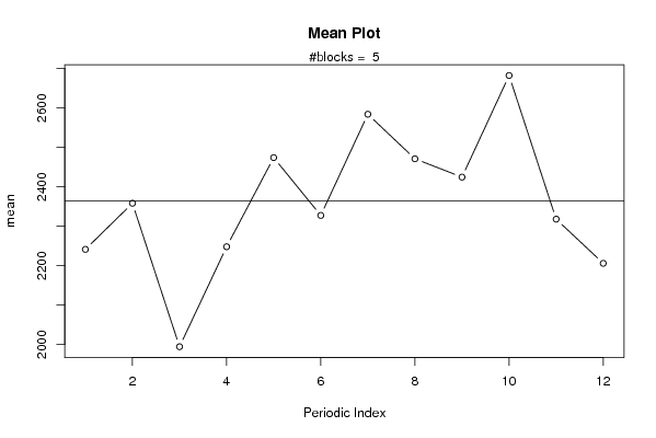
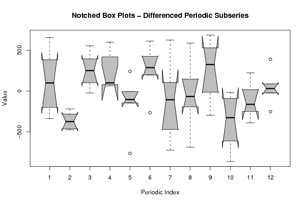
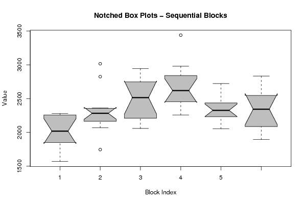
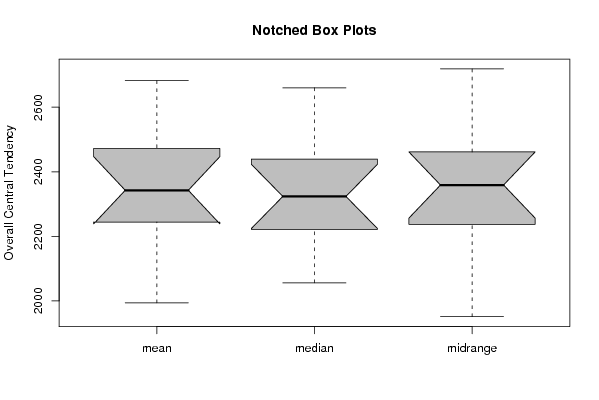
| Title produced by software | Mean Plot | ||||||||||||||||||||
| Date of computation | Fri, 05 Dec 2008 06:08:19 -0700 | ||||||||||||||||||||
| Cite this page as follows | Statistical Computations at FreeStatistics.org, Office for Research Development and Education, URL https://freestatistics.org/blog/index.php?v=date/2008/Dec/05/t12284825264iw2vpgjgqu6sys.htm/, Retrieved Thu, 16 May 2024 21:35:34 +0000 | ||||||||||||||||||||
| Statistical Computations at FreeStatistics.org, Office for Research Development and Education, URL https://freestatistics.org/blog/index.php?pk=29229, Retrieved Thu, 16 May 2024 21:35:34 +0000 | |||||||||||||||||||||
| QR Codes: | |||||||||||||||||||||
|
| |||||||||||||||||||||
| Original text written by user: | |||||||||||||||||||||
| IsPrivate? | No (this computation is public) | ||||||||||||||||||||
| User-defined keywords | |||||||||||||||||||||
| Estimated Impact | 182 | ||||||||||||||||||||
Tree of Dependent Computations | |||||||||||||||||||||
| Family? (F = Feedback message, R = changed R code, M = changed R Module, P = changed Parameters, D = changed Data) | |||||||||||||||||||||
| - [Kendall tau Correlation Matrix] [Kendall Tau Corre...] [2007-11-09 12:45:53] [74be16979710d4c4e7c6647856088456] - RMPD [Mean Plot] [Mean Plot: Bouwve...] [2008-12-05 13:08:19] [b5110a3ab194da7214bdf478e0a05dbd] [Current] | |||||||||||||||||||||
| Feedback Forum | |||||||||||||||||||||
Post a new message | |||||||||||||||||||||
Dataset | |||||||||||||||||||||
| Dataseries X: | |||||||||||||||||||||
2187 1852 1570 1851 1954 1828 2251 2277 2085 2282 2266 1878 2267 2069 1746 2299 2360 2214 2825 2355 2333 3016 2155 2172 2150 2533 2058 2160 2259 2498 2695 2799 2945 2930 2318 2540 2570 2669 2450 2842 3439 2677 2979 2257 2842 2546 2455 2293 2379 2478 2054 2272 2351 2271 2542 2304 2194 2722 2395 2146 1894 2548 2087 2063 2481 2476 2212 2834 2148 2598 | |||||||||||||||||||||
Tables (Output of Computation) | |||||||||||||||||||||
| |||||||||||||||||||||
Figures (Output of Computation) | |||||||||||||||||||||
Input Parameters & R Code | |||||||||||||||||||||
| Parameters (Session): | |||||||||||||||||||||
| par1 = 12 ; | |||||||||||||||||||||
| Parameters (R input): | |||||||||||||||||||||
| par1 = 12 ; | |||||||||||||||||||||
| R code (references can be found in the software module): | |||||||||||||||||||||
par1 <- as.numeric(par1) | |||||||||||||||||||||