Free Statistics
of Irreproducible Research!
Description of Statistical Computation | |||||||||||||||||||||||||||||||||||||||||||||||||||||
|---|---|---|---|---|---|---|---|---|---|---|---|---|---|---|---|---|---|---|---|---|---|---|---|---|---|---|---|---|---|---|---|---|---|---|---|---|---|---|---|---|---|---|---|---|---|---|---|---|---|---|---|---|---|
| Author's title | |||||||||||||||||||||||||||||||||||||||||||||||||||||
| Author | *The author of this computation has been verified* | ||||||||||||||||||||||||||||||||||||||||||||||||||||
| R Software Module | rwasp_edauni.wasp | ||||||||||||||||||||||||||||||||||||||||||||||||||||
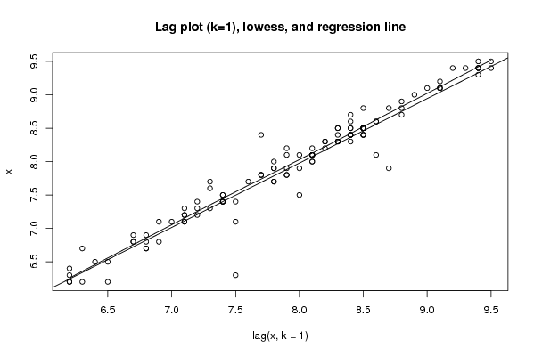
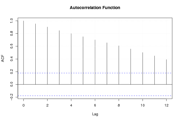
| Title produced by software | Univariate Explorative Data Analysis | ||||||||||||||||||||||||||||||||||||||||||||||||||||
| Date of computation | Fri, 05 Dec 2008 05:38:56 -0700 | ||||||||||||||||||||||||||||||||||||||||||||||||||||
| Cite this page as follows | Statistical Computations at FreeStatistics.org, Office for Research Development and Education, URL https://freestatistics.org/blog/index.php?v=date/2008/Dec/05/t1228480795tpwo8pdcdf44wj4.htm/, Retrieved Thu, 03 Jul 2025 11:30:08 +0000 | ||||||||||||||||||||||||||||||||||||||||||||||||||||
| Statistical Computations at FreeStatistics.org, Office for Research Development and Education, URL https://freestatistics.org/blog/index.php?pk=29215, Retrieved Thu, 03 Jul 2025 11:30:08 +0000 | |||||||||||||||||||||||||||||||||||||||||||||||||||||
| QR Codes: | |||||||||||||||||||||||||||||||||||||||||||||||||||||
|
| |||||||||||||||||||||||||||||||||||||||||||||||||||||
| Original text written by user: | |||||||||||||||||||||||||||||||||||||||||||||||||||||
| IsPrivate? | No (this computation is public) | ||||||||||||||||||||||||||||||||||||||||||||||||||||
| User-defined keywords | |||||||||||||||||||||||||||||||||||||||||||||||||||||
| Estimated Impact | 303 | ||||||||||||||||||||||||||||||||||||||||||||||||||||
Tree of Dependent Computations | |||||||||||||||||||||||||||||||||||||||||||||||||||||
| Family? (F = Feedback message, R = changed R code, M = changed R Module, P = changed Parameters, D = changed Data) | |||||||||||||||||||||||||||||||||||||||||||||||||||||
| - [Univariate Data Series] [Werkloosheidsgraa...] [2008-12-05 10:45:42] [e5d91604aae608e98a8ea24759233f66] - PD [Univariate Data Series] [Inflatie op jaarb...] [2008-12-05 10:52:23] [e5d91604aae608e98a8ea24759233f66] - PD [Univariate Data Series] [Investeringen vol...] [2008-12-05 10:58:14] [e5d91604aae608e98a8ea24759233f66] - RMPD [Central Tendency] [Central Tendency ...] [2008-12-05 11:16:53] [e5d91604aae608e98a8ea24759233f66] - RMP [Univariate Explorative Data Analysis] [EDA Werkloosheids...] [2008-12-05 12:38:56] [55ca0ca4a201c9689dcf5fae352c92eb] [Current] | |||||||||||||||||||||||||||||||||||||||||||||||||||||
| Feedback Forum | |||||||||||||||||||||||||||||||||||||||||||||||||||||
Post a new message | |||||||||||||||||||||||||||||||||||||||||||||||||||||
Dataset | |||||||||||||||||||||||||||||||||||||||||||||||||||||
| Dataseries X: | |||||||||||||||||||||||||||||||||||||||||||||||||||||
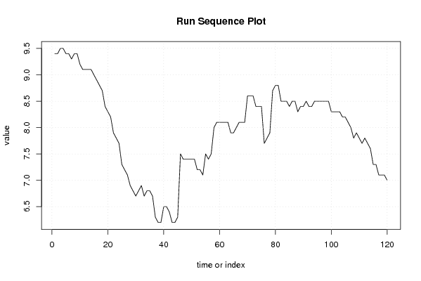
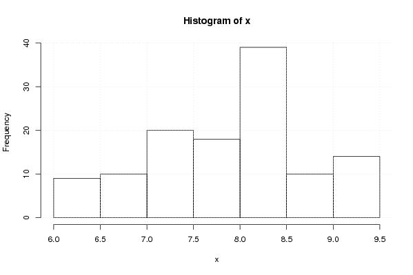
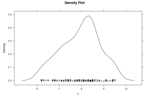
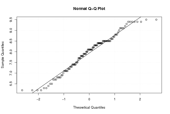
9.4 9.4 9.5 9.5 9.4 9.4 9.3 9.4 9.4 9.2 9.1 9.1 9.1 9.1 9 8.9 8.8 8.7 8.4 8.3 8.2 7.9 7.8 7.7 7.3 7.2 7.1 6.9 6.8 6.7 6.8 6.9 6.7 6.8 6.8 6.7 6.3 6.2 6.2 6.5 6.5 6.4 6.2 6.2 6.3 7.5 7.4 7.4 7.4 7.4 7.4 7.2 7.2 7.1 7.5 7.4 7.5 8 8.1 8.1 8.1 8.1 8.1 7.9 7.9 8 8.1 8.1 8.1 8.6 8.6 8.6 8.4 8.4 8.4 7.7 7.8 7.9 8.7 8.8 8.8 8.5 8.5 8.5 8.4 8.5 8.5 8.3 8.4 8.4 8.5 8.4 8.4 8.5 8.5 8.5 8.5 8.5 8.5 8.3 8.3 8.3 8.3 8.2 8.2 8.1 8 7.8 7.9 7.8 7.7 7.8 7.7 7.6 7.3 7.3 7.1 7.1 7.1 7 | |||||||||||||||||||||||||||||||||||||||||||||||||||||
Tables (Output of Computation) | |||||||||||||||||||||||||||||||||||||||||||||||||||||
| |||||||||||||||||||||||||||||||||||||||||||||||||||||
Figures (Output of Computation) | |||||||||||||||||||||||||||||||||||||||||||||||||||||
Input Parameters & R Code | |||||||||||||||||||||||||||||||||||||||||||||||||||||
| Parameters (Session): | |||||||||||||||||||||||||||||||||||||||||||||||||||||
| par1 = Inflatie indexcijfer der consumptieprijzen ; par2 = http://ecodata.mineco.fgov.be/mdn/ts_structur.jsp?table=EI0_ ; par3 = Economische indicator voor België. Maandelijks, volledige tijdreeks van januari 1998 tot december 2007 - Inflatie op jaarbasis: indexcijfer der consumptieprijzen ; | |||||||||||||||||||||||||||||||||||||||||||||||||||||
| Parameters (R input): | |||||||||||||||||||||||||||||||||||||||||||||||||||||
| par1 = 0 ; par2 = 12 ; | |||||||||||||||||||||||||||||||||||||||||||||||||||||
| R code (references can be found in the software module): | |||||||||||||||||||||||||||||||||||||||||||||||||||||
par1 <- as.numeric(par1) | |||||||||||||||||||||||||||||||||||||||||||||||||||||