Repository of Reproducible Computations

Free Statistics

of Irreproducible Research!

Author's title

Author

*The author of this computation has been verified*

R Software Module

rwasp_autocorrelation.wasp

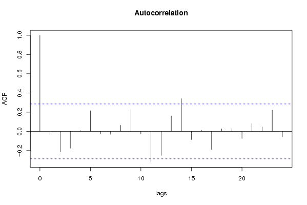
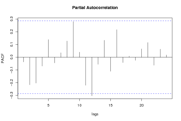
Title produced by software

(Partial) Autocorrelation Function

Date of computation

Fri, 05 Dec 2008 04:21:04 -0700

Cite this page as follows

Statistical Computations at FreeStatistics.org, Office for Research Development and Education, URL https://freestatistics.org/blog/index.php?v=date/2008/Dec/05/t12284761677ykub2o61tcmz7u.htm/, Retrieved Thu, 16 May 2024 12:27:26 +0000

Statistical Computations at FreeStatistics.org, Office for Research Development and Education, URL https://freestatistics.org/blog/index.php?pk=29176, Retrieved Thu, 16 May 2024 12:27:26 +0000

QR Codes:

Paste this QR Code to cite your computation.

Original text written by user:

IsPrivate?

No (this computation is public)

User-defined keywords

Estimated Impact

242

Family? (F = Feedback message, R = changed R code, M = changed R Module, P = changed Parameters, D = changed Data)

-     [Standard Deviation-Mean Plot] [Paper Hoofdstuk 4...] [2008-12-05 10:14:55] [6fea0e9a9b3b29a63badf2c274e82506]
- RMP     [(Partial) Autocorrelation Function] [Paper Hoofdstuk 4...] [2008-12-05 11:21:04] [286e96bd53289970f8e5f25a93fb50b3] [Current]
-   P       [(Partial) Autocorrelation Function] [Paper Hoofdstuk 4...] [2008-12-05 22:37:51] [6fea0e9a9b3b29a63badf2c274e82506] 
-   P       [(Partial) Autocorrelation Function] [Paper Hoofdstuk 4...] [2008-12-05 23:07:43] [6fea0e9a9b3b29a63badf2c274e82506] 
- RMP       [Spectral Analysis] [Paper Hoofdstuk 4...] [2008-12-05 23:23:55] [6fea0e9a9b3b29a63badf2c274e82506] 
-   P         [Spectral Analysis] [Paper Hoofdstuk 4...] [2008-12-06 11:37:54] [6fea0e9a9b3b29a63badf2c274e82506] 
-   P         [Spectral Analysis] [Paper Hoofdstuk 4...] [2008-12-06 11:44:44] [6fea0e9a9b3b29a63badf2c274e82506] 

Feedback Forum

Post a new message

Dataseries X:

Download CSV

Histogram

Boxplots

Summary of computational transaction
Raw Input	view raw input (R code)
Raw Output	view raw output of R engine
Computing time	1 seconds
R Server	'Gwilym Jenkins' @ 72.249.127.135

\begin{tabular}{lllllllll}
\hline
Summary of computational transaction \tabularnewline
Raw Input & view raw input (R code)  \tabularnewline
Raw Output & view raw output of R engine  \tabularnewline
Computing time & 1 seconds \tabularnewline
R Server & 'Gwilym Jenkins' @ 72.249.127.135 \tabularnewline
\hline
\end{tabular}
%Source: https://freestatistics.org/blog/index.php?pk=29176&T=0

[TABLE]
[ROW][C]Summary of computational transaction[/C][/ROW]
[ROW][C]Raw Input[/C][C]view raw input (R code) [/C][/ROW]
[ROW][C]Raw Output[/C][C]view raw output of R engine [/C][/ROW]
[ROW][C]Computing time[/C][C]1 seconds[/C][/ROW]
[ROW][C]R Server[/C][C]'Gwilym Jenkins' @ 72.249.127.135[/C][/ROW]
[/TABLE]
Source: https://freestatistics.org/blog/index.php?pk=29176&T=0

Globally Unique Identifier (entire table): ba.freestatistics.org/blog/index.php?pk=29176&T=0

As an alternative you can also use a QR Code:

The GUIDs for individual cells are displayed in the table below:

Summary of computational transaction
Raw Input	view raw input (R code)
Raw Output	view raw output of R engine
Computing time	1 seconds
R Server	'Gwilym Jenkins' @ 72.249.127.135

Autocorrelation Function
Time lag k	ACF(k)	T-STAT	P-value
1	-0.037447	-0.2567	0.399255
2	-0.215341	-1.4763	0.073266
3	-0.175986	-1.2065	0.116831
4	0.008426	0.0578	0.47709
5	0.215569	1.4779	0.073057
6	-0.024342	-0.1669	0.434091
7	-0.030351	-0.2081	0.418033
8	0.063867	0.4378	0.33175
9	0.228324	1.5653	0.062109
10	-0.02612	-0.1791	0.429327
11	-0.321615	-2.2049	0.016196
12	-0.249649	-1.7115	0.04679
13	0.161284	1.1057	0.137241
14	0.340655	2.3354	0.011921
15	-0.085017	-0.5828	0.281392
16	0.011751	0.0806	0.468068
17	-0.188428	-1.2918	0.101372
18	0.02709	0.1857	0.426732
19	0.028905	0.1982	0.421885
20	-0.074468	-0.5105	0.306036
21	0.080967	0.5551	0.290736
22	0.0464	0.3181	0.375908
23	0.222049	1.5223	0.067318
24	-0.056105	-0.3846	0.351121

\begin{tabular}{lllllllll}
\hline
Autocorrelation Function \tabularnewline
Time lag k & ACF(k) & T-STAT & P-value \tabularnewline
1 & -0.037447 & -0.2567 & 0.399255 \tabularnewline
2 & -0.215341 & -1.4763 & 0.073266 \tabularnewline
3 & -0.175986 & -1.2065 & 0.116831 \tabularnewline
4 & 0.008426 & 0.0578 & 0.47709 \tabularnewline
5 & 0.215569 & 1.4779 & 0.073057 \tabularnewline
6 & -0.024342 & -0.1669 & 0.434091 \tabularnewline
7 & -0.030351 & -0.2081 & 0.418033 \tabularnewline
8 & 0.063867 & 0.4378 & 0.33175 \tabularnewline
9 & 0.228324 & 1.5653 & 0.062109 \tabularnewline
10 & -0.02612 & -0.1791 & 0.429327 \tabularnewline
11 & -0.321615 & -2.2049 & 0.016196 \tabularnewline
12 & -0.249649 & -1.7115 & 0.04679 \tabularnewline
13 & 0.161284 & 1.1057 & 0.137241 \tabularnewline
14 & 0.340655 & 2.3354 & 0.011921 \tabularnewline
15 & -0.085017 & -0.5828 & 0.281392 \tabularnewline
16 & 0.011751 & 0.0806 & 0.468068 \tabularnewline
17 & -0.188428 & -1.2918 & 0.101372 \tabularnewline
18 & 0.02709 & 0.1857 & 0.426732 \tabularnewline
19 & 0.028905 & 0.1982 & 0.421885 \tabularnewline
20 & -0.074468 & -0.5105 & 0.306036 \tabularnewline
21 & 0.080967 & 0.5551 & 0.290736 \tabularnewline
22 & 0.0464 & 0.3181 & 0.375908 \tabularnewline
23 & 0.222049 & 1.5223 & 0.067318 \tabularnewline
24 & -0.056105 & -0.3846 & 0.351121 \tabularnewline
\hline
\end{tabular}
%Source: https://freestatistics.org/blog/index.php?pk=29176&T=1

[TABLE]
[ROW][C]Autocorrelation Function[/C][/ROW]
[ROW][C]Time lag k[/C][C]ACF(k)[/C][C]T-STAT[/C][C]P-value[/C][/ROW]
[ROW][C]1[/C][C]-0.037447[/C][C]-0.2567[/C][C]0.399255[/C][/ROW]
[ROW][C]2[/C][C]-0.215341[/C][C]-1.4763[/C][C]0.073266[/C][/ROW]
[ROW][C]3[/C][C]-0.175986[/C][C]-1.2065[/C][C]0.116831[/C][/ROW]
[ROW][C]4[/C][C]0.008426[/C][C]0.0578[/C][C]0.47709[/C][/ROW]
[ROW][C]5[/C][C]0.215569[/C][C]1.4779[/C][C]0.073057[/C][/ROW]
[ROW][C]6[/C][C]-0.024342[/C][C]-0.1669[/C][C]0.434091[/C][/ROW]
[ROW][C]7[/C][C]-0.030351[/C][C]-0.2081[/C][C]0.418033[/C][/ROW]
[ROW][C]8[/C][C]0.063867[/C][C]0.4378[/C][C]0.33175[/C][/ROW]
[ROW][C]9[/C][C]0.228324[/C][C]1.5653[/C][C]0.062109[/C][/ROW]
[ROW][C]10[/C][C]-0.02612[/C][C]-0.1791[/C][C]0.429327[/C][/ROW]
[ROW][C]11[/C][C]-0.321615[/C][C]-2.2049[/C][C]0.016196[/C][/ROW]
[ROW][C]12[/C][C]-0.249649[/C][C]-1.7115[/C][C]0.04679[/C][/ROW]
[ROW][C]13[/C][C]0.161284[/C][C]1.1057[/C][C]0.137241[/C][/ROW]
[ROW][C]14[/C][C]0.340655[/C][C]2.3354[/C][C]0.011921[/C][/ROW]
[ROW][C]15[/C][C]-0.085017[/C][C]-0.5828[/C][C]0.281392[/C][/ROW]
[ROW][C]16[/C][C]0.011751[/C][C]0.0806[/C][C]0.468068[/C][/ROW]
[ROW][C]17[/C][C]-0.188428[/C][C]-1.2918[/C][C]0.101372[/C][/ROW]
[ROW][C]18[/C][C]0.02709[/C][C]0.1857[/C][C]0.426732[/C][/ROW]
[ROW][C]19[/C][C]0.028905[/C][C]0.1982[/C][C]0.421885[/C][/ROW]
[ROW][C]20[/C][C]-0.074468[/C][C]-0.5105[/C][C]0.306036[/C][/ROW]
[ROW][C]21[/C][C]0.080967[/C][C]0.5551[/C][C]0.290736[/C][/ROW]
[ROW][C]22[/C][C]0.0464[/C][C]0.3181[/C][C]0.375908[/C][/ROW]
[ROW][C]23[/C][C]0.222049[/C][C]1.5223[/C][C]0.067318[/C][/ROW]
[ROW][C]24[/C][C]-0.056105[/C][C]-0.3846[/C][C]0.351121[/C][/ROW]
[/TABLE]
Source: https://freestatistics.org/blog/index.php?pk=29176&T=1

Globally Unique Identifier (entire table): ba.freestatistics.org/blog/index.php?pk=29176&T=1

As an alternative you can also use a QR Code:

The GUIDs for individual cells are displayed in the table below:

Autocorrelation Function
Time lag k	ACF(k)	T-STAT	P-value
1	-0.037447	-0.2567	0.399255
2	-0.215341	-1.4763	0.073266
3	-0.175986	-1.2065	0.116831
4	0.008426	0.0578	0.47709
5	0.215569	1.4779	0.073057
6	-0.024342	-0.1669	0.434091
7	-0.030351	-0.2081	0.418033
8	0.063867	0.4378	0.33175
9	0.228324	1.5653	0.062109
10	-0.02612	-0.1791	0.429327
11	-0.321615	-2.2049	0.016196
12	-0.249649	-1.7115	0.04679
13	0.161284	1.1057	0.137241
14	0.340655	2.3354	0.011921
15	-0.085017	-0.5828	0.281392
16	0.011751	0.0806	0.468068
17	-0.188428	-1.2918	0.101372
18	0.02709	0.1857	0.426732
19	0.028905	0.1982	0.421885
20	-0.074468	-0.5105	0.306036
21	0.080967	0.5551	0.290736
22	0.0464	0.3181	0.375908
23	0.222049	1.5223	0.067318
24	-0.056105	-0.3846	0.351121

Partial Autocorrelation Function
Time lag k	PACF(k)	T-STAT	P-value
1	-0.037447	-0.2567	0.399255
2	-0.217047	-1.488	0.071715
3	-0.203802	-1.3972	0.084458
4	-0.069899	-0.4792	0.317007
5	0.138802	0.9516	0.173089
6	-0.044947	-0.3081	0.379667
7	0.035303	0.242	0.404907
8	0.127326	0.8729	0.193578
9	0.28033	1.9218	0.03035
10	0.039932	0.2738	0.392734
11	-0.22077	-1.5135	0.068421
12	-0.303368	-2.0798	0.021512
13	-0.056056	-0.3843	0.351245
14	0.133316	0.914	0.1827
15	-0.111017	-0.7611	0.225202
16	0.216905	1.487	0.071843
17	-0.042398	-0.2907	0.386294
18	0.008535	0.0585	0.476793
19	-0.02482	-0.1702	0.43281
20	0.06599	0.4524	0.32653
21	0.115839	0.7942	0.215549
22	-0.063406	-0.4347	0.332889
23	0.063496	0.4353	0.332667
24	0.017674	0.1212	0.452037

\begin{tabular}{lllllllll}
\hline
Partial Autocorrelation Function \tabularnewline
Time lag k & PACF(k) & T-STAT & P-value \tabularnewline
1 & -0.037447 & -0.2567 & 0.399255 \tabularnewline
2 & -0.217047 & -1.488 & 0.071715 \tabularnewline
3 & -0.203802 & -1.3972 & 0.084458 \tabularnewline
4 & -0.069899 & -0.4792 & 0.317007 \tabularnewline
5 & 0.138802 & 0.9516 & 0.173089 \tabularnewline
6 & -0.044947 & -0.3081 & 0.379667 \tabularnewline
7 & 0.035303 & 0.242 & 0.404907 \tabularnewline
8 & 0.127326 & 0.8729 & 0.193578 \tabularnewline
9 & 0.28033 & 1.9218 & 0.03035 \tabularnewline
10 & 0.039932 & 0.2738 & 0.392734 \tabularnewline
11 & -0.22077 & -1.5135 & 0.068421 \tabularnewline
12 & -0.303368 & -2.0798 & 0.021512 \tabularnewline
13 & -0.056056 & -0.3843 & 0.351245 \tabularnewline
14 & 0.133316 & 0.914 & 0.1827 \tabularnewline
15 & -0.111017 & -0.7611 & 0.225202 \tabularnewline
16 & 0.216905 & 1.487 & 0.071843 \tabularnewline
17 & -0.042398 & -0.2907 & 0.386294 \tabularnewline
18 & 0.008535 & 0.0585 & 0.476793 \tabularnewline
19 & -0.02482 & -0.1702 & 0.43281 \tabularnewline
20 & 0.06599 & 0.4524 & 0.32653 \tabularnewline
21 & 0.115839 & 0.7942 & 0.215549 \tabularnewline
22 & -0.063406 & -0.4347 & 0.332889 \tabularnewline
23 & 0.063496 & 0.4353 & 0.332667 \tabularnewline
24 & 0.017674 & 0.1212 & 0.452037 \tabularnewline
\hline
\end{tabular}
%Source: https://freestatistics.org/blog/index.php?pk=29176&T=2

[TABLE]
[ROW][C]Partial Autocorrelation Function[/C][/ROW]
[ROW][C]Time lag k[/C][C]PACF(k)[/C][C]T-STAT[/C][C]P-value[/C][/ROW]
[ROW][C]1[/C][C]-0.037447[/C][C]-0.2567[/C][C]0.399255[/C][/ROW]
[ROW][C]2[/C][C]-0.217047[/C][C]-1.488[/C][C]0.071715[/C][/ROW]
[ROW][C]3[/C][C]-0.203802[/C][C]-1.3972[/C][C]0.084458[/C][/ROW]
[ROW][C]4[/C][C]-0.069899[/C][C]-0.4792[/C][C]0.317007[/C][/ROW]
[ROW][C]5[/C][C]0.138802[/C][C]0.9516[/C][C]0.173089[/C][/ROW]
[ROW][C]6[/C][C]-0.044947[/C][C]-0.3081[/C][C]0.379667[/C][/ROW]
[ROW][C]7[/C][C]0.035303[/C][C]0.242[/C][C]0.404907[/C][/ROW]
[ROW][C]8[/C][C]0.127326[/C][C]0.8729[/C][C]0.193578[/C][/ROW]
[ROW][C]9[/C][C]0.28033[/C][C]1.9218[/C][C]0.03035[/C][/ROW]
[ROW][C]10[/C][C]0.039932[/C][C]0.2738[/C][C]0.392734[/C][/ROW]
[ROW][C]11[/C][C]-0.22077[/C][C]-1.5135[/C][C]0.068421[/C][/ROW]
[ROW][C]12[/C][C]-0.303368[/C][C]-2.0798[/C][C]0.021512[/C][/ROW]
[ROW][C]13[/C][C]-0.056056[/C][C]-0.3843[/C][C]0.351245[/C][/ROW]
[ROW][C]14[/C][C]0.133316[/C][C]0.914[/C][C]0.1827[/C][/ROW]
[ROW][C]15[/C][C]-0.111017[/C][C]-0.7611[/C][C]0.225202[/C][/ROW]
[ROW][C]16[/C][C]0.216905[/C][C]1.487[/C][C]0.071843[/C][/ROW]
[ROW][C]17[/C][C]-0.042398[/C][C]-0.2907[/C][C]0.386294[/C][/ROW]
[ROW][C]18[/C][C]0.008535[/C][C]0.0585[/C][C]0.476793[/C][/ROW]
[ROW][C]19[/C][C]-0.02482[/C][C]-0.1702[/C][C]0.43281[/C][/ROW]
[ROW][C]20[/C][C]0.06599[/C][C]0.4524[/C][C]0.32653[/C][/ROW]
[ROW][C]21[/C][C]0.115839[/C][C]0.7942[/C][C]0.215549[/C][/ROW]
[ROW][C]22[/C][C]-0.063406[/C][C]-0.4347[/C][C]0.332889[/C][/ROW]
[ROW][C]23[/C][C]0.063496[/C][C]0.4353[/C][C]0.332667[/C][/ROW]
[ROW][C]24[/C][C]0.017674[/C][C]0.1212[/C][C]0.452037[/C][/ROW]
[/TABLE]
Source: https://freestatistics.org/blog/index.php?pk=29176&T=2

Globally Unique Identifier (entire table): ba.freestatistics.org/blog/index.php?pk=29176&T=2

As an alternative you can also use a QR Code:

The GUIDs for individual cells are displayed in the table below:

Partial Autocorrelation Function
Time lag k	PACF(k)	T-STAT	P-value
1	-0.037447	-0.2567	0.399255
2	-0.217047	-1.488	0.071715
3	-0.203802	-1.3972	0.084458
4	-0.069899	-0.4792	0.317007
5	0.138802	0.9516	0.173089
6	-0.044947	-0.3081	0.379667
7	0.035303	0.242	0.404907
8	0.127326	0.8729	0.193578
9	0.28033	1.9218	0.03035
10	0.039932	0.2738	0.392734
11	-0.22077	-1.5135	0.068421
12	-0.303368	-2.0798	0.021512
13	-0.056056	-0.3843	0.351245
14	0.133316	0.914	0.1827
15	-0.111017	-0.7611	0.225202
16	0.216905	1.487	0.071843
17	-0.042398	-0.2907	0.386294
18	0.008535	0.0585	0.476793
19	-0.02482	-0.1702	0.43281
20	0.06599	0.4524	0.32653
21	0.115839	0.7942	0.215549
22	-0.063406	-0.4347	0.332889
23	0.063496	0.4353	0.332667
24	0.017674	0.1212	0.452037

Figure 1

PNG link

Postscript link

PDF link

Figure 2

PNG link

Postscript link

PDF link

Parameters (Session):

par1 = 24 ; par2 = 1 ; par3 = 1 ; par4 = 1 ; par5 = 12 ;

Parameters (R input):

par1 = 24 ; par2 = 1 ; par3 = 1 ; par4 = 1 ; par5 = 12 ;

R code (references can be found in the software module):

if (par1 == 'Default') {
par1 = 10*log10(length(x))
} else {
par1 <- as.numeric(par1)
}
par2 <- as.numeric(par2)
par3 <- as.numeric(par3)
par4 <- as.numeric(par4)
par5 <- as.numeric(par5)
if (par2 == 0) {
x <- log(x)
} else {
x <- (x ^ par2 - 1) / par2
}
if (par3 > 0) x <- diff(x,lag=1,difference=par3)
if (par4 > 0) x <- diff(x,lag=par5,difference=par4)
bitmap(file='pic1.png')
racf <- acf(x,par1,main='Autocorrelation',xlab='lags',ylab='ACF')
dev.off()
bitmap(file='pic2.png')
rpacf <- pacf(x,par1,main='Partial Autocorrelation',xlab='lags',ylab='PACF')
dev.off()
(myacf <- c(racf$acf))
(mypacf <- c(rpacf$acf))
lengthx <- length(x)
sqrtn <- sqrt(lengthx)
load(file='createtable')
a<-table.start()
a<-table.row.start(a)
a<-table.element(a,'Autocorrelation Function',4,TRUE)
a<-table.row.end(a)
a<-table.row.start(a)
a<-table.element(a,'Time lag k',header=TRUE)
a<-table.element(a,hyperlink('basics.htm','ACF(k)','click here for more information about the Autocorrelation Function'),header=TRUE)
a<-table.element(a,'T-STAT',header=TRUE)
a<-table.element(a,'P-value',header=TRUE)
a<-table.row.end(a)
for (i in 2:(par1+1)) {
a<-table.row.start(a)
a<-table.element(a,i-1,header=TRUE)
a<-table.element(a,round(myacf[i],6))
mytstat <- myacf[i]*sqrtn
a<-table.element(a,round(mytstat,4))
a<-table.element(a,round(1-pt(abs(mytstat),lengthx),6))
a<-table.row.end(a)
}
a<-table.end(a)
table.save(a,file='mytable.tab')
a<-table.start()
a<-table.row.start(a)
a<-table.element(a,'Partial Autocorrelation Function',4,TRUE)
a<-table.row.end(a)
a<-table.row.start(a)
a<-table.element(a,'Time lag k',header=TRUE)
a<-table.element(a,hyperlink('basics.htm','PACF(k)','click here for more information about the Partial Autocorrelation Function'),header=TRUE)
a<-table.element(a,'T-STAT',header=TRUE)
a<-table.element(a,'P-value',header=TRUE)
a<-table.row.end(a)
for (i in 1:par1) {
a<-table.row.start(a)
a<-table.element(a,i,header=TRUE)
a<-table.element(a,round(mypacf[i],6))
mytstat <- mypacf[i]*sqrtn
a<-table.element(a,round(mytstat,4))
a<-table.element(a,round(1-pt(abs(mytstat),lengthx),6))
a<-table.row.end(a)
}
a<-table.end(a)
table.save(a,file='mytable1.tab')

Free Statistics

Description of Statistical Computation

Tree of Dependent Computations

Dataset

Tables (Output of Computation)

Figures (Output of Computation)

Input Parameters & R Code