Free Statistics

of Irreproducible Research!

Author's title

Autocorrelation werkloosheid 31/12/2001 - 31/12/2007 met d en D gelijk aan ...

Author

*Unverified author*

R Software Module

rwasp_autocorrelation.wasp

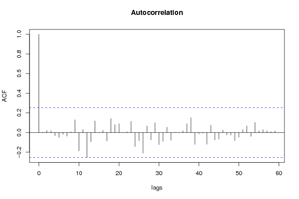
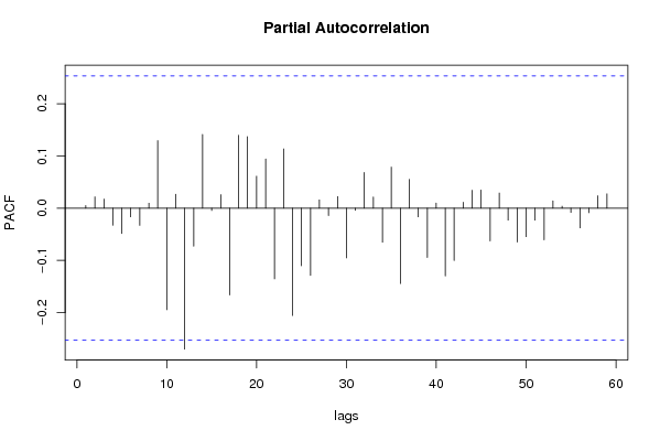
Title produced by software

(Partial) Autocorrelation Function

Date of computation

Wed, 03 Dec 2008 12:06:20 -0700

Cite this page as follows

Statistical Computations at FreeStatistics.org, Office for Research Development and Education, URL https://freestatistics.org/blog/index.php?v=date/2008/Dec/03/t1228331532xjqvz8gzcbtpjsm.htm/, Retrieved Fri, 17 May 2024 12:47:07 +0000

Statistical Computations at FreeStatistics.org, Office for Research Development and Education, URL https://freestatistics.org/blog/index.php?pk=28850, Retrieved Fri, 17 May 2024 12:47:07 +0000

QR Codes:

Paste this QR Code to cite your computation.

Original text written by user:

IsPrivate?

No (this computation is public)

User-defined keywords

Estimated Impact

183

Family? (F = Feedback message, R = changed R code, M = changed R Module, P = changed Parameters, D = changed Data)

-     [Univariate Data Series] [data set] [2008-12-01 19:54:57] [b98453cac15ba1066b407e146608df68]
-   PD  [Univariate Data Series] [Werkloosheids Bel...] [2008-12-03 18:39:41] [74be16979710d4c4e7c6647856088456]
-   PD    [Univariate Data Series] [Werkloosheids Bel...] [2008-12-03 18:47:55] [74be16979710d4c4e7c6647856088456]
- RMP       [Variance Reduction Matrix] [VRM werkloosheid ...] [2008-12-03 18:51:43] [74be16979710d4c4e7c6647856088456]
- RMP         [(Partial) Autocorrelation Function] [Autocorrelation w...] [2008-12-03 18:58:20] [27f46dbe13ae2811dfd3a6f3c54d4d50]
-   P           [(Partial) Autocorrelation Function] [Autocorrelation w...] [2008-12-03 19:01:56] [27f46dbe13ae2811dfd3a6f3c54d4d50]
-   P               [(Partial) Autocorrelation Function] [Autocorrelation w...] [2008-12-03 19:06:20] [822e74e765918799ae89051d24799c03] [Current]
- RMP                 [Spectral Analysis] [Spectral analysis...] [2008-12-03 19:13:53] [27f46dbe13ae2811dfd3a6f3c54d4d50] 
-   P                   [Spectral Analysis] [Spectral analysis...] [2008-12-03 19:19:15] [27f46dbe13ae2811dfd3a6f3c54d4d50] 
-                         [Spectral Analysis] [Spectral analysis...] [2008-12-03 19:22:31] [27f46dbe13ae2811dfd3a6f3c54d4d50] 

Feedback Forum

Post a new message

Dataseries X:

Download CSV

Histogram

Boxplots

Summary of computational transaction
Raw Input	view raw input (R code)
Raw Output	view raw output of R engine
Computing time	1 seconds
R Server	'Gwilym Jenkins' @ 72.249.127.135

\begin{tabular}{lllllllll}
\hline
Summary of computational transaction \tabularnewline
Raw Input & view raw input (R code)  \tabularnewline
Raw Output & view raw output of R engine  \tabularnewline
Computing time & 1 seconds \tabularnewline
R Server & 'Gwilym Jenkins' @ 72.249.127.135 \tabularnewline
\hline
\end{tabular}
%Source: https://freestatistics.org/blog/index.php?pk=28850&T=0

[TABLE]
[ROW][C]Summary of computational transaction[/C][/ROW]
[ROW][C]Raw Input[/C][C]view raw input (R code) [/C][/ROW]
[ROW][C]Raw Output[/C][C]view raw output of R engine [/C][/ROW]
[ROW][C]Computing time[/C][C]1 seconds[/C][/ROW]
[ROW][C]R Server[/C][C]'Gwilym Jenkins' @ 72.249.127.135[/C][/ROW]
[/TABLE]
Source: https://freestatistics.org/blog/index.php?pk=28850&T=0

Globally Unique Identifier (entire table): ba.freestatistics.org/blog/index.php?pk=28850&T=0

As an alternative you can also use a QR Code:

The GUIDs for individual cells are displayed in the table below:

Summary of computational transaction
Raw Input	view raw input (R code)
Raw Output	view raw output of R engine
Computing time	1 seconds
R Server	'Gwilym Jenkins' @ 72.249.127.135

Autocorrelation Function
Time lag k	ACF(k)	T-STAT	P-value
1	0.005184	0.0402	0.484051
2	0.021784	0.1687	0.433287
3	0.017768	0.1376	0.445497
4	-0.032044	-0.2482	0.402409
5	-0.04808	-0.3724	0.355445
6	-0.01805	-0.1398	0.444637
7	-0.036369	-0.2817	0.389568
8	0.007763	0.0601	0.476127
9	0.129654	1.0043	0.159636
10	-0.187147	-1.4496	0.076183
11	0.03003	0.2326	0.408429
12	-0.254069	-1.968	0.026847
13	-0.093433	-0.7237	0.236023
14	0.118641	0.919	0.180891
15	0.001142	0.0088	0.496487
16	0.022979	0.178	0.429664
17	-0.085321	-0.6609	0.255605
18	0.141996	1.0999	0.137886
19	0.08097	0.6272	0.266458
20	0.089578	0.6939	0.245221
21	-0.002605	-0.0202	0.491983
22	0.008353	0.0647	0.474312
23	0.1148	0.8892	0.188714
24	-0.142775	-1.1059	0.136586
25	-0.083333	-0.6455	0.260533
26	-0.209428	-1.6222	0.055
27	0.067983	0.5266	0.300209
28	-0.075302	-0.5833	0.280943
29	0.101048	0.7827	0.218438
30	-0.122818	-0.9513	0.172624
31	-0.089498	-0.6932	0.245415
32	0.054956	0.4257	0.33593
33	-0.079264	-0.614	0.270776
34	0.004083	0.0316	0.487438
35	0.001209	0.0094	0.49628
36	0.020024	0.1551	0.438629
37	0.090478	0.7008	0.243056
38	0.151598	1.1743	0.122462
39	-0.119809	-0.928	0.178553
40	-0.012893	-0.0999	0.460391
41	-0.006299	-0.0488	0.480625
42	-0.118695	-0.9194	0.180783
43	0.074711	0.5787	0.282475
44	-0.075557	-0.5853	0.280282
45	-0.065136	-0.5045	0.307865
46	0.026873	0.2082	0.417904
47	-0.024281	-0.1881	0.425723
48	-0.026148	-0.2025	0.420089
49	-0.08328	-0.6451	0.260667
50	-0.046737	-0.362	0.359305
51	0.031305	0.2425	0.404614
52	0.068251	0.5287	0.299491
53	-0.039377	-0.305	0.380706
54	0.103465	0.8014	0.213021
55	0.01766	0.1368	0.445824
56	0.028821	0.2232	0.412051
57	0.018963	0.1469	0.441856
58	0.00924	0.0716	0.47159
59	0.016438	0.1273	0.449552
60	NA	NA	NA

\begin{tabular}{lllllllll}
\hline
Autocorrelation Function \tabularnewline
Time lag k & ACF(k) & T-STAT & P-value \tabularnewline
1 & 0.005184 & 0.0402 & 0.484051 \tabularnewline
2 & 0.021784 & 0.1687 & 0.433287 \tabularnewline
3 & 0.017768 & 0.1376 & 0.445497 \tabularnewline
4 & -0.032044 & -0.2482 & 0.402409 \tabularnewline
5 & -0.04808 & -0.3724 & 0.355445 \tabularnewline
6 & -0.01805 & -0.1398 & 0.444637 \tabularnewline
7 & -0.036369 & -0.2817 & 0.389568 \tabularnewline
8 & 0.007763 & 0.0601 & 0.476127 \tabularnewline
9 & 0.129654 & 1.0043 & 0.159636 \tabularnewline
10 & -0.187147 & -1.4496 & 0.076183 \tabularnewline
11 & 0.03003 & 0.2326 & 0.408429 \tabularnewline
12 & -0.254069 & -1.968 & 0.026847 \tabularnewline
13 & -0.093433 & -0.7237 & 0.236023 \tabularnewline
14 & 0.118641 & 0.919 & 0.180891 \tabularnewline
15 & 0.001142 & 0.0088 & 0.496487 \tabularnewline
16 & 0.022979 & 0.178 & 0.429664 \tabularnewline
17 & -0.085321 & -0.6609 & 0.255605 \tabularnewline
18 & 0.141996 & 1.0999 & 0.137886 \tabularnewline
19 & 0.08097 & 0.6272 & 0.266458 \tabularnewline
20 & 0.089578 & 0.6939 & 0.245221 \tabularnewline
21 & -0.002605 & -0.0202 & 0.491983 \tabularnewline
22 & 0.008353 & 0.0647 & 0.474312 \tabularnewline
23 & 0.1148 & 0.8892 & 0.188714 \tabularnewline
24 & -0.142775 & -1.1059 & 0.136586 \tabularnewline
25 & -0.083333 & -0.6455 & 0.260533 \tabularnewline
26 & -0.209428 & -1.6222 & 0.055 \tabularnewline
27 & 0.067983 & 0.5266 & 0.300209 \tabularnewline
28 & -0.075302 & -0.5833 & 0.280943 \tabularnewline
29 & 0.101048 & 0.7827 & 0.218438 \tabularnewline
30 & -0.122818 & -0.9513 & 0.172624 \tabularnewline
31 & -0.089498 & -0.6932 & 0.245415 \tabularnewline
32 & 0.054956 & 0.4257 & 0.33593 \tabularnewline
33 & -0.079264 & -0.614 & 0.270776 \tabularnewline
34 & 0.004083 & 0.0316 & 0.487438 \tabularnewline
35 & 0.001209 & 0.0094 & 0.49628 \tabularnewline
36 & 0.020024 & 0.1551 & 0.438629 \tabularnewline
37 & 0.090478 & 0.7008 & 0.243056 \tabularnewline
38 & 0.151598 & 1.1743 & 0.122462 \tabularnewline
39 & -0.119809 & -0.928 & 0.178553 \tabularnewline
40 & -0.012893 & -0.0999 & 0.460391 \tabularnewline
41 & -0.006299 & -0.0488 & 0.480625 \tabularnewline
42 & -0.118695 & -0.9194 & 0.180783 \tabularnewline
43 & 0.074711 & 0.5787 & 0.282475 \tabularnewline
44 & -0.075557 & -0.5853 & 0.280282 \tabularnewline
45 & -0.065136 & -0.5045 & 0.307865 \tabularnewline
46 & 0.026873 & 0.2082 & 0.417904 \tabularnewline
47 & -0.024281 & -0.1881 & 0.425723 \tabularnewline
48 & -0.026148 & -0.2025 & 0.420089 \tabularnewline
49 & -0.08328 & -0.6451 & 0.260667 \tabularnewline
50 & -0.046737 & -0.362 & 0.359305 \tabularnewline
51 & 0.031305 & 0.2425 & 0.404614 \tabularnewline
52 & 0.068251 & 0.5287 & 0.299491 \tabularnewline
53 & -0.039377 & -0.305 & 0.380706 \tabularnewline
54 & 0.103465 & 0.8014 & 0.213021 \tabularnewline
55 & 0.01766 & 0.1368 & 0.445824 \tabularnewline
56 & 0.028821 & 0.2232 & 0.412051 \tabularnewline
57 & 0.018963 & 0.1469 & 0.441856 \tabularnewline
58 & 0.00924 & 0.0716 & 0.47159 \tabularnewline
59 & 0.016438 & 0.1273 & 0.449552 \tabularnewline
60 & NA & NA & NA \tabularnewline
\hline
\end{tabular}
%Source: https://freestatistics.org/blog/index.php?pk=28850&T=1

[TABLE]
[ROW][C]Autocorrelation Function[/C][/ROW]
[ROW][C]Time lag k[/C][C]ACF(k)[/C][C]T-STAT[/C][C]P-value[/C][/ROW]
[ROW][C]1[/C][C]0.005184[/C][C]0.0402[/C][C]0.484051[/C][/ROW]
[ROW][C]2[/C][C]0.021784[/C][C]0.1687[/C][C]0.433287[/C][/ROW]
[ROW][C]3[/C][C]0.017768[/C][C]0.1376[/C][C]0.445497[/C][/ROW]
[ROW][C]4[/C][C]-0.032044[/C][C]-0.2482[/C][C]0.402409[/C][/ROW]
[ROW][C]5[/C][C]-0.04808[/C][C]-0.3724[/C][C]0.355445[/C][/ROW]
[ROW][C]6[/C][C]-0.01805[/C][C]-0.1398[/C][C]0.444637[/C][/ROW]
[ROW][C]7[/C][C]-0.036369[/C][C]-0.2817[/C][C]0.389568[/C][/ROW]
[ROW][C]8[/C][C]0.007763[/C][C]0.0601[/C][C]0.476127[/C][/ROW]
[ROW][C]9[/C][C]0.129654[/C][C]1.0043[/C][C]0.159636[/C][/ROW]
[ROW][C]10[/C][C]-0.187147[/C][C]-1.4496[/C][C]0.076183[/C][/ROW]
[ROW][C]11[/C][C]0.03003[/C][C]0.2326[/C][C]0.408429[/C][/ROW]
[ROW][C]12[/C][C]-0.254069[/C][C]-1.968[/C][C]0.026847[/C][/ROW]
[ROW][C]13[/C][C]-0.093433[/C][C]-0.7237[/C][C]0.236023[/C][/ROW]
[ROW][C]14[/C][C]0.118641[/C][C]0.919[/C][C]0.180891[/C][/ROW]
[ROW][C]15[/C][C]0.001142[/C][C]0.0088[/C][C]0.496487[/C][/ROW]
[ROW][C]16[/C][C]0.022979[/C][C]0.178[/C][C]0.429664[/C][/ROW]
[ROW][C]17[/C][C]-0.085321[/C][C]-0.6609[/C][C]0.255605[/C][/ROW]
[ROW][C]18[/C][C]0.141996[/C][C]1.0999[/C][C]0.137886[/C][/ROW]
[ROW][C]19[/C][C]0.08097[/C][C]0.6272[/C][C]0.266458[/C][/ROW]
[ROW][C]20[/C][C]0.089578[/C][C]0.6939[/C][C]0.245221[/C][/ROW]
[ROW][C]21[/C][C]-0.002605[/C][C]-0.0202[/C][C]0.491983[/C][/ROW]
[ROW][C]22[/C][C]0.008353[/C][C]0.0647[/C][C]0.474312[/C][/ROW]
[ROW][C]23[/C][C]0.1148[/C][C]0.8892[/C][C]0.188714[/C][/ROW]
[ROW][C]24[/C][C]-0.142775[/C][C]-1.1059[/C][C]0.136586[/C][/ROW]
[ROW][C]25[/C][C]-0.083333[/C][C]-0.6455[/C][C]0.260533[/C][/ROW]
[ROW][C]26[/C][C]-0.209428[/C][C]-1.6222[/C][C]0.055[/C][/ROW]
[ROW][C]27[/C][C]0.067983[/C][C]0.5266[/C][C]0.300209[/C][/ROW]
[ROW][C]28[/C][C]-0.075302[/C][C]-0.5833[/C][C]0.280943[/C][/ROW]
[ROW][C]29[/C][C]0.101048[/C][C]0.7827[/C][C]0.218438[/C][/ROW]
[ROW][C]30[/C][C]-0.122818[/C][C]-0.9513[/C][C]0.172624[/C][/ROW]
[ROW][C]31[/C][C]-0.089498[/C][C]-0.6932[/C][C]0.245415[/C][/ROW]
[ROW][C]32[/C][C]0.054956[/C][C]0.4257[/C][C]0.33593[/C][/ROW]
[ROW][C]33[/C][C]-0.079264[/C][C]-0.614[/C][C]0.270776[/C][/ROW]
[ROW][C]34[/C][C]0.004083[/C][C]0.0316[/C][C]0.487438[/C][/ROW]
[ROW][C]35[/C][C]0.001209[/C][C]0.0094[/C][C]0.49628[/C][/ROW]
[ROW][C]36[/C][C]0.020024[/C][C]0.1551[/C][C]0.438629[/C][/ROW]
[ROW][C]37[/C][C]0.090478[/C][C]0.7008[/C][C]0.243056[/C][/ROW]
[ROW][C]38[/C][C]0.151598[/C][C]1.1743[/C][C]0.122462[/C][/ROW]
[ROW][C]39[/C][C]-0.119809[/C][C]-0.928[/C][C]0.178553[/C][/ROW]
[ROW][C]40[/C][C]-0.012893[/C][C]-0.0999[/C][C]0.460391[/C][/ROW]
[ROW][C]41[/C][C]-0.006299[/C][C]-0.0488[/C][C]0.480625[/C][/ROW]
[ROW][C]42[/C][C]-0.118695[/C][C]-0.9194[/C][C]0.180783[/C][/ROW]
[ROW][C]43[/C][C]0.074711[/C][C]0.5787[/C][C]0.282475[/C][/ROW]
[ROW][C]44[/C][C]-0.075557[/C][C]-0.5853[/C][C]0.280282[/C][/ROW]
[ROW][C]45[/C][C]-0.065136[/C][C]-0.5045[/C][C]0.307865[/C][/ROW]
[ROW][C]46[/C][C]0.026873[/C][C]0.2082[/C][C]0.417904[/C][/ROW]
[ROW][C]47[/C][C]-0.024281[/C][C]-0.1881[/C][C]0.425723[/C][/ROW]
[ROW][C]48[/C][C]-0.026148[/C][C]-0.2025[/C][C]0.420089[/C][/ROW]
[ROW][C]49[/C][C]-0.08328[/C][C]-0.6451[/C][C]0.260667[/C][/ROW]
[ROW][C]50[/C][C]-0.046737[/C][C]-0.362[/C][C]0.359305[/C][/ROW]
[ROW][C]51[/C][C]0.031305[/C][C]0.2425[/C][C]0.404614[/C][/ROW]
[ROW][C]52[/C][C]0.068251[/C][C]0.5287[/C][C]0.299491[/C][/ROW]
[ROW][C]53[/C][C]-0.039377[/C][C]-0.305[/C][C]0.380706[/C][/ROW]
[ROW][C]54[/C][C]0.103465[/C][C]0.8014[/C][C]0.213021[/C][/ROW]
[ROW][C]55[/C][C]0.01766[/C][C]0.1368[/C][C]0.445824[/C][/ROW]
[ROW][C]56[/C][C]0.028821[/C][C]0.2232[/C][C]0.412051[/C][/ROW]
[ROW][C]57[/C][C]0.018963[/C][C]0.1469[/C][C]0.441856[/C][/ROW]
[ROW][C]58[/C][C]0.00924[/C][C]0.0716[/C][C]0.47159[/C][/ROW]
[ROW][C]59[/C][C]0.016438[/C][C]0.1273[/C][C]0.449552[/C][/ROW]
[ROW][C]60[/C][C]NA[/C][C]NA[/C][C]NA[/C][/ROW]
[/TABLE]
Source: https://freestatistics.org/blog/index.php?pk=28850&T=1

Globally Unique Identifier (entire table): ba.freestatistics.org/blog/index.php?pk=28850&T=1

As an alternative you can also use a QR Code:

The GUIDs for individual cells are displayed in the table below:

Autocorrelation Function
Time lag k	ACF(k)	T-STAT	P-value
1	0.005184	0.0402	0.484051
2	0.021784	0.1687	0.433287
3	0.017768	0.1376	0.445497
4	-0.032044	-0.2482	0.402409
5	-0.04808	-0.3724	0.355445
6	-0.01805	-0.1398	0.444637
7	-0.036369	-0.2817	0.389568
8	0.007763	0.0601	0.476127
9	0.129654	1.0043	0.159636
10	-0.187147	-1.4496	0.076183
11	0.03003	0.2326	0.408429
12	-0.254069	-1.968	0.026847
13	-0.093433	-0.7237	0.236023
14	0.118641	0.919	0.180891
15	0.001142	0.0088	0.496487
16	0.022979	0.178	0.429664
17	-0.085321	-0.6609	0.255605
18	0.141996	1.0999	0.137886
19	0.08097	0.6272	0.266458
20	0.089578	0.6939	0.245221
21	-0.002605	-0.0202	0.491983
22	0.008353	0.0647	0.474312
23	0.1148	0.8892	0.188714
24	-0.142775	-1.1059	0.136586
25	-0.083333	-0.6455	0.260533
26	-0.209428	-1.6222	0.055
27	0.067983	0.5266	0.300209
28	-0.075302	-0.5833	0.280943
29	0.101048	0.7827	0.218438
30	-0.122818	-0.9513	0.172624
31	-0.089498	-0.6932	0.245415
32	0.054956	0.4257	0.33593
33	-0.079264	-0.614	0.270776
34	0.004083	0.0316	0.487438
35	0.001209	0.0094	0.49628
36	0.020024	0.1551	0.438629
37	0.090478	0.7008	0.243056
38	0.151598	1.1743	0.122462
39	-0.119809	-0.928	0.178553
40	-0.012893	-0.0999	0.460391
41	-0.006299	-0.0488	0.480625
42	-0.118695	-0.9194	0.180783
43	0.074711	0.5787	0.282475
44	-0.075557	-0.5853	0.280282
45	-0.065136	-0.5045	0.307865
46	0.026873	0.2082	0.417904
47	-0.024281	-0.1881	0.425723
48	-0.026148	-0.2025	0.420089
49	-0.08328	-0.6451	0.260667
50	-0.046737	-0.362	0.359305
51	0.031305	0.2425	0.404614
52	0.068251	0.5287	0.299491
53	-0.039377	-0.305	0.380706
54	0.103465	0.8014	0.213021
55	0.01766	0.1368	0.445824
56	0.028821	0.2232	0.412051
57	0.018963	0.1469	0.441856
58	0.00924	0.0716	0.47159
59	0.016438	0.1273	0.449552
60	NA	NA	NA

Partial Autocorrelation Function
Time lag k	PACF(k)	T-STAT	P-value
1	0.005184	0.0402	0.484051
2	0.021757	0.1685	0.433366
3	0.017553	0.136	0.446151
4	-0.032717	-0.2534	0.400404
5	-0.048616	-0.3766	0.353908
6	-0.016574	-0.1284	0.449139
7	-0.033049	-0.256	0.399416
8	0.009521	0.0737	0.470728
9	0.129409	1.0024	0.160089
10	-0.19453	-1.5068	0.068551
11	0.026714	0.2069	0.418386
12	-0.269778	-2.0897	0.020447
13	-0.072731	-0.5634	0.28764
14	0.141085	1.0928	0.139417
15	-0.004521	-0.035	0.48609
16	0.025815	0.2	0.421092
17	-0.166293	-1.2881	0.101329
18	0.139595	1.0813	0.141945
19	0.137084	1.0618	0.146281
20	0.061297	0.4748	0.318326
21	0.09417	0.7294	0.234287
22	-0.135236	-1.0475	0.149528
23	0.113453	0.8788	0.191506
24	-0.205595	-1.5925	0.05826
25	-0.110191	-0.8535	0.198379
26	-0.128745	-0.9973	0.161324
27	0.015824	0.1226	0.451428
28	-0.014199	-0.11	0.456396
29	0.022196	0.1719	0.432036
30	-0.095232	-0.7377	0.231796
31	-0.004197	-0.0325	0.487087
32	0.068417	0.53	0.29905
33	0.021511	0.1666	0.434113
34	-0.065092	-0.5042	0.307984
35	0.078754	0.61	0.272075
36	-0.144284	-1.1176	0.134092
37	0.055061	0.4265	0.335634
38	-0.01656	-0.1283	0.449182
39	-0.094298	-0.7304	0.233985
40	0.009778	0.0757	0.469938
41	-0.129791	-1.0054	0.159382
42	-0.100341	-0.7772	0.220035
43	0.011307	0.0876	0.465251
44	0.034257	0.2654	0.395823
45	0.034739	0.2691	0.394391
46	-0.062722	-0.4858	0.314425
47	0.029006	0.2247	0.411495
48	-0.022994	-0.1781	0.429617
49	-0.064781	-0.5018	0.308826
50	-0.054646	-0.4233	0.336799
51	-0.022867	-0.1771	0.430001
52	-0.060691	-0.4701	0.319991
53	0.013996	0.1084	0.457015
54	0.003859	0.0299	0.488125
55	-0.008201	-0.0635	0.474779
56	-0.037645	-0.2916	0.3858
57	-0.00858	-0.0665	0.473615
58	0.023707	0.1836	0.427461
59	0.027377	0.2121	0.416388
60	NA	NA	NA

\begin{tabular}{lllllllll}
\hline
Partial Autocorrelation Function \tabularnewline
Time lag k & PACF(k) & T-STAT & P-value \tabularnewline
1 & 0.005184 & 0.0402 & 0.484051 \tabularnewline
2 & 0.021757 & 0.1685 & 0.433366 \tabularnewline
3 & 0.017553 & 0.136 & 0.446151 \tabularnewline
4 & -0.032717 & -0.2534 & 0.400404 \tabularnewline
5 & -0.048616 & -0.3766 & 0.353908 \tabularnewline
6 & -0.016574 & -0.1284 & 0.449139 \tabularnewline
7 & -0.033049 & -0.256 & 0.399416 \tabularnewline
8 & 0.009521 & 0.0737 & 0.470728 \tabularnewline
9 & 0.129409 & 1.0024 & 0.160089 \tabularnewline
10 & -0.19453 & -1.5068 & 0.068551 \tabularnewline
11 & 0.026714 & 0.2069 & 0.418386 \tabularnewline
12 & -0.269778 & -2.0897 & 0.020447 \tabularnewline
13 & -0.072731 & -0.5634 & 0.28764 \tabularnewline
14 & 0.141085 & 1.0928 & 0.139417 \tabularnewline
15 & -0.004521 & -0.035 & 0.48609 \tabularnewline
16 & 0.025815 & 0.2 & 0.421092 \tabularnewline
17 & -0.166293 & -1.2881 & 0.101329 \tabularnewline
18 & 0.139595 & 1.0813 & 0.141945 \tabularnewline
19 & 0.137084 & 1.0618 & 0.146281 \tabularnewline
20 & 0.061297 & 0.4748 & 0.318326 \tabularnewline
21 & 0.09417 & 0.7294 & 0.234287 \tabularnewline
22 & -0.135236 & -1.0475 & 0.149528 \tabularnewline
23 & 0.113453 & 0.8788 & 0.191506 \tabularnewline
24 & -0.205595 & -1.5925 & 0.05826 \tabularnewline
25 & -0.110191 & -0.8535 & 0.198379 \tabularnewline
26 & -0.128745 & -0.9973 & 0.161324 \tabularnewline
27 & 0.015824 & 0.1226 & 0.451428 \tabularnewline
28 & -0.014199 & -0.11 & 0.456396 \tabularnewline
29 & 0.022196 & 0.1719 & 0.432036 \tabularnewline
30 & -0.095232 & -0.7377 & 0.231796 \tabularnewline
31 & -0.004197 & -0.0325 & 0.487087 \tabularnewline
32 & 0.068417 & 0.53 & 0.29905 \tabularnewline
33 & 0.021511 & 0.1666 & 0.434113 \tabularnewline
34 & -0.065092 & -0.5042 & 0.307984 \tabularnewline
35 & 0.078754 & 0.61 & 0.272075 \tabularnewline
36 & -0.144284 & -1.1176 & 0.134092 \tabularnewline
37 & 0.055061 & 0.4265 & 0.335634 \tabularnewline
38 & -0.01656 & -0.1283 & 0.449182 \tabularnewline
39 & -0.094298 & -0.7304 & 0.233985 \tabularnewline
40 & 0.009778 & 0.0757 & 0.469938 \tabularnewline
41 & -0.129791 & -1.0054 & 0.159382 \tabularnewline
42 & -0.100341 & -0.7772 & 0.220035 \tabularnewline
43 & 0.011307 & 0.0876 & 0.465251 \tabularnewline
44 & 0.034257 & 0.2654 & 0.395823 \tabularnewline
45 & 0.034739 & 0.2691 & 0.394391 \tabularnewline
46 & -0.062722 & -0.4858 & 0.314425 \tabularnewline
47 & 0.029006 & 0.2247 & 0.411495 \tabularnewline
48 & -0.022994 & -0.1781 & 0.429617 \tabularnewline
49 & -0.064781 & -0.5018 & 0.308826 \tabularnewline
50 & -0.054646 & -0.4233 & 0.336799 \tabularnewline
51 & -0.022867 & -0.1771 & 0.430001 \tabularnewline
52 & -0.060691 & -0.4701 & 0.319991 \tabularnewline
53 & 0.013996 & 0.1084 & 0.457015 \tabularnewline
54 & 0.003859 & 0.0299 & 0.488125 \tabularnewline
55 & -0.008201 & -0.0635 & 0.474779 \tabularnewline
56 & -0.037645 & -0.2916 & 0.3858 \tabularnewline
57 & -0.00858 & -0.0665 & 0.473615 \tabularnewline
58 & 0.023707 & 0.1836 & 0.427461 \tabularnewline
59 & 0.027377 & 0.2121 & 0.416388 \tabularnewline
60 & NA & NA & NA \tabularnewline
\hline
\end{tabular}
%Source: https://freestatistics.org/blog/index.php?pk=28850&T=2

[TABLE]
[ROW][C]Partial Autocorrelation Function[/C][/ROW]
[ROW][C]Time lag k[/C][C]PACF(k)[/C][C]T-STAT[/C][C]P-value[/C][/ROW]
[ROW][C]1[/C][C]0.005184[/C][C]0.0402[/C][C]0.484051[/C][/ROW]
[ROW][C]2[/C][C]0.021757[/C][C]0.1685[/C][C]0.433366[/C][/ROW]
[ROW][C]3[/C][C]0.017553[/C][C]0.136[/C][C]0.446151[/C][/ROW]
[ROW][C]4[/C][C]-0.032717[/C][C]-0.2534[/C][C]0.400404[/C][/ROW]
[ROW][C]5[/C][C]-0.048616[/C][C]-0.3766[/C][C]0.353908[/C][/ROW]
[ROW][C]6[/C][C]-0.016574[/C][C]-0.1284[/C][C]0.449139[/C][/ROW]
[ROW][C]7[/C][C]-0.033049[/C][C]-0.256[/C][C]0.399416[/C][/ROW]
[ROW][C]8[/C][C]0.009521[/C][C]0.0737[/C][C]0.470728[/C][/ROW]
[ROW][C]9[/C][C]0.129409[/C][C]1.0024[/C][C]0.160089[/C][/ROW]
[ROW][C]10[/C][C]-0.19453[/C][C]-1.5068[/C][C]0.068551[/C][/ROW]
[ROW][C]11[/C][C]0.026714[/C][C]0.2069[/C][C]0.418386[/C][/ROW]
[ROW][C]12[/C][C]-0.269778[/C][C]-2.0897[/C][C]0.020447[/C][/ROW]
[ROW][C]13[/C][C]-0.072731[/C][C]-0.5634[/C][C]0.28764[/C][/ROW]
[ROW][C]14[/C][C]0.141085[/C][C]1.0928[/C][C]0.139417[/C][/ROW]
[ROW][C]15[/C][C]-0.004521[/C][C]-0.035[/C][C]0.48609[/C][/ROW]
[ROW][C]16[/C][C]0.025815[/C][C]0.2[/C][C]0.421092[/C][/ROW]
[ROW][C]17[/C][C]-0.166293[/C][C]-1.2881[/C][C]0.101329[/C][/ROW]
[ROW][C]18[/C][C]0.139595[/C][C]1.0813[/C][C]0.141945[/C][/ROW]
[ROW][C]19[/C][C]0.137084[/C][C]1.0618[/C][C]0.146281[/C][/ROW]
[ROW][C]20[/C][C]0.061297[/C][C]0.4748[/C][C]0.318326[/C][/ROW]
[ROW][C]21[/C][C]0.09417[/C][C]0.7294[/C][C]0.234287[/C][/ROW]
[ROW][C]22[/C][C]-0.135236[/C][C]-1.0475[/C][C]0.149528[/C][/ROW]
[ROW][C]23[/C][C]0.113453[/C][C]0.8788[/C][C]0.191506[/C][/ROW]
[ROW][C]24[/C][C]-0.205595[/C][C]-1.5925[/C][C]0.05826[/C][/ROW]
[ROW][C]25[/C][C]-0.110191[/C][C]-0.8535[/C][C]0.198379[/C][/ROW]
[ROW][C]26[/C][C]-0.128745[/C][C]-0.9973[/C][C]0.161324[/C][/ROW]
[ROW][C]27[/C][C]0.015824[/C][C]0.1226[/C][C]0.451428[/C][/ROW]
[ROW][C]28[/C][C]-0.014199[/C][C]-0.11[/C][C]0.456396[/C][/ROW]
[ROW][C]29[/C][C]0.022196[/C][C]0.1719[/C][C]0.432036[/C][/ROW]
[ROW][C]30[/C][C]-0.095232[/C][C]-0.7377[/C][C]0.231796[/C][/ROW]
[ROW][C]31[/C][C]-0.004197[/C][C]-0.0325[/C][C]0.487087[/C][/ROW]
[ROW][C]32[/C][C]0.068417[/C][C]0.53[/C][C]0.29905[/C][/ROW]
[ROW][C]33[/C][C]0.021511[/C][C]0.1666[/C][C]0.434113[/C][/ROW]
[ROW][C]34[/C][C]-0.065092[/C][C]-0.5042[/C][C]0.307984[/C][/ROW]
[ROW][C]35[/C][C]0.078754[/C][C]0.61[/C][C]0.272075[/C][/ROW]
[ROW][C]36[/C][C]-0.144284[/C][C]-1.1176[/C][C]0.134092[/C][/ROW]
[ROW][C]37[/C][C]0.055061[/C][C]0.4265[/C][C]0.335634[/C][/ROW]
[ROW][C]38[/C][C]-0.01656[/C][C]-0.1283[/C][C]0.449182[/C][/ROW]
[ROW][C]39[/C][C]-0.094298[/C][C]-0.7304[/C][C]0.233985[/C][/ROW]
[ROW][C]40[/C][C]0.009778[/C][C]0.0757[/C][C]0.469938[/C][/ROW]
[ROW][C]41[/C][C]-0.129791[/C][C]-1.0054[/C][C]0.159382[/C][/ROW]
[ROW][C]42[/C][C]-0.100341[/C][C]-0.7772[/C][C]0.220035[/C][/ROW]
[ROW][C]43[/C][C]0.011307[/C][C]0.0876[/C][C]0.465251[/C][/ROW]
[ROW][C]44[/C][C]0.034257[/C][C]0.2654[/C][C]0.395823[/C][/ROW]
[ROW][C]45[/C][C]0.034739[/C][C]0.2691[/C][C]0.394391[/C][/ROW]
[ROW][C]46[/C][C]-0.062722[/C][C]-0.4858[/C][C]0.314425[/C][/ROW]
[ROW][C]47[/C][C]0.029006[/C][C]0.2247[/C][C]0.411495[/C][/ROW]
[ROW][C]48[/C][C]-0.022994[/C][C]-0.1781[/C][C]0.429617[/C][/ROW]
[ROW][C]49[/C][C]-0.064781[/C][C]-0.5018[/C][C]0.308826[/C][/ROW]
[ROW][C]50[/C][C]-0.054646[/C][C]-0.4233[/C][C]0.336799[/C][/ROW]
[ROW][C]51[/C][C]-0.022867[/C][C]-0.1771[/C][C]0.430001[/C][/ROW]
[ROW][C]52[/C][C]-0.060691[/C][C]-0.4701[/C][C]0.319991[/C][/ROW]
[ROW][C]53[/C][C]0.013996[/C][C]0.1084[/C][C]0.457015[/C][/ROW]
[ROW][C]54[/C][C]0.003859[/C][C]0.0299[/C][C]0.488125[/C][/ROW]
[ROW][C]55[/C][C]-0.008201[/C][C]-0.0635[/C][C]0.474779[/C][/ROW]
[ROW][C]56[/C][C]-0.037645[/C][C]-0.2916[/C][C]0.3858[/C][/ROW]
[ROW][C]57[/C][C]-0.00858[/C][C]-0.0665[/C][C]0.473615[/C][/ROW]
[ROW][C]58[/C][C]0.023707[/C][C]0.1836[/C][C]0.427461[/C][/ROW]
[ROW][C]59[/C][C]0.027377[/C][C]0.2121[/C][C]0.416388[/C][/ROW]
[ROW][C]60[/C][C]NA[/C][C]NA[/C][C]NA[/C][/ROW]
[/TABLE]
Source: https://freestatistics.org/blog/index.php?pk=28850&T=2

Globally Unique Identifier (entire table): ba.freestatistics.org/blog/index.php?pk=28850&T=2

As an alternative you can also use a QR Code:

The GUIDs for individual cells are displayed in the table below:

Partial Autocorrelation Function
Time lag k	PACF(k)	T-STAT	P-value
1	0.005184	0.0402	0.484051
2	0.021757	0.1685	0.433366
3	0.017553	0.136	0.446151
4	-0.032717	-0.2534	0.400404
5	-0.048616	-0.3766	0.353908
6	-0.016574	-0.1284	0.449139
7	-0.033049	-0.256	0.399416
8	0.009521	0.0737	0.470728
9	0.129409	1.0024	0.160089
10	-0.19453	-1.5068	0.068551
11	0.026714	0.2069	0.418386
12	-0.269778	-2.0897	0.020447
13	-0.072731	-0.5634	0.28764
14	0.141085	1.0928	0.139417
15	-0.004521	-0.035	0.48609
16	0.025815	0.2	0.421092
17	-0.166293	-1.2881	0.101329
18	0.139595	1.0813	0.141945
19	0.137084	1.0618	0.146281
20	0.061297	0.4748	0.318326
21	0.09417	0.7294	0.234287
22	-0.135236	-1.0475	0.149528
23	0.113453	0.8788	0.191506
24	-0.205595	-1.5925	0.05826
25	-0.110191	-0.8535	0.198379
26	-0.128745	-0.9973	0.161324
27	0.015824	0.1226	0.451428
28	-0.014199	-0.11	0.456396
29	0.022196	0.1719	0.432036
30	-0.095232	-0.7377	0.231796
31	-0.004197	-0.0325	0.487087
32	0.068417	0.53	0.29905
33	0.021511	0.1666	0.434113
34	-0.065092	-0.5042	0.307984
35	0.078754	0.61	0.272075
36	-0.144284	-1.1176	0.134092
37	0.055061	0.4265	0.335634
38	-0.01656	-0.1283	0.449182
39	-0.094298	-0.7304	0.233985
40	0.009778	0.0757	0.469938
41	-0.129791	-1.0054	0.159382
42	-0.100341	-0.7772	0.220035
43	0.011307	0.0876	0.465251
44	0.034257	0.2654	0.395823
45	0.034739	0.2691	0.394391
46	-0.062722	-0.4858	0.314425
47	0.029006	0.2247	0.411495
48	-0.022994	-0.1781	0.429617
49	-0.064781	-0.5018	0.308826
50	-0.054646	-0.4233	0.336799
51	-0.022867	-0.1771	0.430001
52	-0.060691	-0.4701	0.319991
53	0.013996	0.1084	0.457015
54	0.003859	0.0299	0.488125
55	-0.008201	-0.0635	0.474779
56	-0.037645	-0.2916	0.3858
57	-0.00858	-0.0665	0.473615
58	0.023707	0.1836	0.427461
59	0.027377	0.2121	0.416388
60	NA	NA	NA

Figure 1

PNG link

Postscript link

PDF link

Figure 2

PNG link

Postscript link

PDF link

Parameters (Session):

par1 = 60 ; par2 = 1 ; par3 = 1 ; par4 = 1 ; par5 = 12 ;

Parameters (R input):

par1 = 60 ; par2 = 1 ; par3 = 1 ; par4 = 1 ; par5 = 12 ;

R code (references can be found in the software module):

if (par1 == 'Default') {
par1 = 10*log10(length(x))
} else {
par1 <- as.numeric(par1)
}
par2 <- as.numeric(par2)
par3 <- as.numeric(par3)
par4 <- as.numeric(par4)
par5 <- as.numeric(par5)
if (par2 == 0) {
x <- log(x)
} else {
x <- (x ^ par2 - 1) / par2
}
if (par3 > 0) x <- diff(x,lag=1,difference=par3)
if (par4 > 0) x <- diff(x,lag=par5,difference=par4)
bitmap(file='pic1.png')
racf <- acf(x,par1,main='Autocorrelation',xlab='lags',ylab='ACF')
dev.off()
bitmap(file='pic2.png')
rpacf <- pacf(x,par1,main='Partial Autocorrelation',xlab='lags',ylab='PACF')
dev.off()
(myacf <- c(racf$acf))
(mypacf <- c(rpacf$acf))
lengthx <- length(x)
sqrtn <- sqrt(lengthx)
load(file='createtable')
a<-table.start()
a<-table.row.start(a)
a<-table.element(a,'Autocorrelation Function',4,TRUE)
a<-table.row.end(a)
a<-table.row.start(a)
a<-table.element(a,'Time lag k',header=TRUE)
a<-table.element(a,hyperlink('basics.htm','ACF(k)','click here for more information about the Autocorrelation Function'),header=TRUE)
a<-table.element(a,'T-STAT',header=TRUE)
a<-table.element(a,'P-value',header=TRUE)
a<-table.row.end(a)
for (i in 2:(par1+1)) {
a<-table.row.start(a)
a<-table.element(a,i-1,header=TRUE)
a<-table.element(a,round(myacf[i],6))
mytstat <- myacf[i]*sqrtn
a<-table.element(a,round(mytstat,4))
a<-table.element(a,round(1-pt(abs(mytstat),lengthx),6))
a<-table.row.end(a)
}
a<-table.end(a)
table.save(a,file='mytable.tab')
a<-table.start()
a<-table.row.start(a)
a<-table.element(a,'Partial Autocorrelation Function',4,TRUE)
a<-table.row.end(a)
a<-table.row.start(a)
a<-table.element(a,'Time lag k',header=TRUE)
a<-table.element(a,hyperlink('basics.htm','PACF(k)','click here for more information about the Partial Autocorrelation Function'),header=TRUE)
a<-table.element(a,'T-STAT',header=TRUE)
a<-table.element(a,'P-value',header=TRUE)
a<-table.row.end(a)
for (i in 1:par1) {
a<-table.row.start(a)
a<-table.element(a,i,header=TRUE)
a<-table.element(a,round(mypacf[i],6))
mytstat <- mypacf[i]*sqrtn
a<-table.element(a,round(mytstat,4))
a<-table.element(a,round(1-pt(abs(mytstat),lengthx),6))
a<-table.row.end(a)
}
a<-table.end(a)
table.save(a,file='mytable1.tab')

Free Statistics

Description of Statistical Computation

Autocorrelation werkloosheid 31/12/2001 - 31/12/2007 met d en D gelijk aan ...

Tree of Dependent Computations

Dataset

Tables (Output of Computation)

Figures (Output of Computation)

Input Parameters & R Code