Repository of Reproducible Computations

Free Statistics

of Irreproducible Research!

Author's title

Author

*The author of this computation has been verified*

R Software Module

rwasp_autocorrelation.wasp

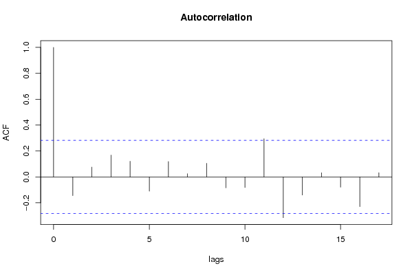
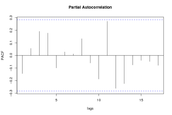
Title produced by software

(Partial) Autocorrelation Function

Date of computation

Wed, 03 Dec 2008 06:25:43 -0700

Cite this page as follows

Statistical Computations at FreeStatistics.org, Office for Research Development and Education, URL https://freestatistics.org/blog/index.php?v=date/2008/Dec/03/t1228310770fyvp823m23hdhvi.htm/, Retrieved Fri, 17 May 2024 19:14:29 +0000

Statistical Computations at FreeStatistics.org, Office for Research Development and Education, URL https://freestatistics.org/blog/index.php?pk=28693, Retrieved Fri, 17 May 2024 19:14:29 +0000

QR Codes:

Paste this QR Code to cite your computation.

Original text written by user:

IsPrivate?

No (this computation is public)

User-defined keywords

Estimated Impact

191

Family? (F = Feedback message, R = changed R code, M = changed R Module, P = changed Parameters, D = changed Data)

F     [Univariate Data Series] [Airline data] [2007-10-18 09:58:47] [42daae401fd3def69a25014f2252b4c2]
- RMPD  [Standard Deviation-Mean Plot] [q5] [2008-12-03 13:15:06] [3ffd109c9e040b1ae7e5dbe576d4698c]
- RMPD    [(Partial) Autocorrelation Function] [q8] [2008-12-03 13:16:51] [3ffd109c9e040b1ae7e5dbe576d4698c]
-   P       [(Partial) Autocorrelation Function] [q8] [2008-12-03 13:23:01] [3ffd109c9e040b1ae7e5dbe576d4698c]
-   P           [(Partial) Autocorrelation Function] [q8] [2008-12-03 13:25:43] [962e6c9020896982bc8283b8971710a9] [Current]
- RMP             [Spectral Analysis] [q8] [2008-12-03 13:33:46] [3ffd109c9e040b1ae7e5dbe576d4698c] 

Feedback Forum

Post a new message

Dataseries X:

Download CSV

Histogram

Boxplots

Summary of computational transaction
Raw Input	view raw input (R code)
Raw Output	view raw output of R engine
Computing time	1 seconds
R Server	'George Udny Yule' @ 72.249.76.132

\begin{tabular}{lllllllll}
\hline
Summary of computational transaction \tabularnewline
Raw Input & view raw input (R code)  \tabularnewline
Raw Output & view raw output of R engine  \tabularnewline
Computing time & 1 seconds \tabularnewline
R Server & 'George Udny Yule' @ 72.249.76.132 \tabularnewline
\hline
\end{tabular}
%Source: https://freestatistics.org/blog/index.php?pk=28693&T=0

[TABLE]
[ROW][C]Summary of computational transaction[/C][/ROW]
[ROW][C]Raw Input[/C][C]view raw input (R code) [/C][/ROW]
[ROW][C]Raw Output[/C][C]view raw output of R engine [/C][/ROW]
[ROW][C]Computing time[/C][C]1 seconds[/C][/ROW]
[ROW][C]R Server[/C][C]'George Udny Yule' @ 72.249.76.132[/C][/ROW]
[/TABLE]
Source: https://freestatistics.org/blog/index.php?pk=28693&T=0

Globally Unique Identifier (entire table): ba.freestatistics.org/blog/index.php?pk=28693&T=0

As an alternative you can also use a QR Code:

The GUIDs for individual cells are displayed in the table below:

Summary of computational transaction
Raw Input	view raw input (R code)
Raw Output	view raw output of R engine
Computing time	1 seconds
R Server	'George Udny Yule' @ 72.249.76.132

Autocorrelation Function
Time lag k	ACF(k)	T-STAT	P-value
1	-0.14455	-1.0015	0.16081
2	0.075879	0.5257	0.300756
3	0.168527	1.1676	0.12437
4	0.121016	0.8384	0.202974
5	-0.110538	-0.7658	0.223764
6	0.118631	0.8219	0.207598
7	0.024556	0.1701	0.432813
8	0.105117	0.7283	0.234993
9	-0.084558	-0.5858	0.280366
10	-0.081611	-0.5654	0.287213
11	0.294689	2.0417	0.023351
12	-0.315137	-2.1833	0.016966
13	-0.14042	-0.9729	0.16775
14	0.031456	0.2179	0.414203
15	-0.079751	-0.5525	0.291575
16	-0.229645	-1.591	0.059084
17	0.032718	0.2267	0.410819

\begin{tabular}{lllllllll}
\hline
Autocorrelation Function \tabularnewline
Time lag k & ACF(k) & T-STAT & P-value \tabularnewline
1 & -0.14455 & -1.0015 & 0.16081 \tabularnewline
2 & 0.075879 & 0.5257 & 0.300756 \tabularnewline
3 & 0.168527 & 1.1676 & 0.12437 \tabularnewline
4 & 0.121016 & 0.8384 & 0.202974 \tabularnewline
5 & -0.110538 & -0.7658 & 0.223764 \tabularnewline
6 & 0.118631 & 0.8219 & 0.207598 \tabularnewline
7 & 0.024556 & 0.1701 & 0.432813 \tabularnewline
8 & 0.105117 & 0.7283 & 0.234993 \tabularnewline
9 & -0.084558 & -0.5858 & 0.280366 \tabularnewline
10 & -0.081611 & -0.5654 & 0.287213 \tabularnewline
11 & 0.294689 & 2.0417 & 0.023351 \tabularnewline
12 & -0.315137 & -2.1833 & 0.016966 \tabularnewline
13 & -0.14042 & -0.9729 & 0.16775 \tabularnewline
14 & 0.031456 & 0.2179 & 0.414203 \tabularnewline
15 & -0.079751 & -0.5525 & 0.291575 \tabularnewline
16 & -0.229645 & -1.591 & 0.059084 \tabularnewline
17 & 0.032718 & 0.2267 & 0.410819 \tabularnewline
\hline
\end{tabular}
%Source: https://freestatistics.org/blog/index.php?pk=28693&T=1

[TABLE]
[ROW][C]Autocorrelation Function[/C][/ROW]
[ROW][C]Time lag k[/C][C]ACF(k)[/C][C]T-STAT[/C][C]P-value[/C][/ROW]
[ROW][C]1[/C][C]-0.14455[/C][C]-1.0015[/C][C]0.16081[/C][/ROW]
[ROW][C]2[/C][C]0.075879[/C][C]0.5257[/C][C]0.300756[/C][/ROW]
[ROW][C]3[/C][C]0.168527[/C][C]1.1676[/C][C]0.12437[/C][/ROW]
[ROW][C]4[/C][C]0.121016[/C][C]0.8384[/C][C]0.202974[/C][/ROW]
[ROW][C]5[/C][C]-0.110538[/C][C]-0.7658[/C][C]0.223764[/C][/ROW]
[ROW][C]6[/C][C]0.118631[/C][C]0.8219[/C][C]0.207598[/C][/ROW]
[ROW][C]7[/C][C]0.024556[/C][C]0.1701[/C][C]0.432813[/C][/ROW]
[ROW][C]8[/C][C]0.105117[/C][C]0.7283[/C][C]0.234993[/C][/ROW]
[ROW][C]9[/C][C]-0.084558[/C][C]-0.5858[/C][C]0.280366[/C][/ROW]
[ROW][C]10[/C][C]-0.081611[/C][C]-0.5654[/C][C]0.287213[/C][/ROW]
[ROW][C]11[/C][C]0.294689[/C][C]2.0417[/C][C]0.023351[/C][/ROW]
[ROW][C]12[/C][C]-0.315137[/C][C]-2.1833[/C][C]0.016966[/C][/ROW]
[ROW][C]13[/C][C]-0.14042[/C][C]-0.9729[/C][C]0.16775[/C][/ROW]
[ROW][C]14[/C][C]0.031456[/C][C]0.2179[/C][C]0.414203[/C][/ROW]
[ROW][C]15[/C][C]-0.079751[/C][C]-0.5525[/C][C]0.291575[/C][/ROW]
[ROW][C]16[/C][C]-0.229645[/C][C]-1.591[/C][C]0.059084[/C][/ROW]
[ROW][C]17[/C][C]0.032718[/C][C]0.2267[/C][C]0.410819[/C][/ROW]
[/TABLE]
Source: https://freestatistics.org/blog/index.php?pk=28693&T=1

Globally Unique Identifier (entire table): ba.freestatistics.org/blog/index.php?pk=28693&T=1

As an alternative you can also use a QR Code:

The GUIDs for individual cells are displayed in the table below:

Autocorrelation Function
Time lag k	ACF(k)	T-STAT	P-value
1	-0.14455	-1.0015	0.16081
2	0.075879	0.5257	0.300756
3	0.168527	1.1676	0.12437
4	0.121016	0.8384	0.202974
5	-0.110538	-0.7658	0.223764
6	0.118631	0.8219	0.207598
7	0.024556	0.1701	0.432813
8	0.105117	0.7283	0.234993
9	-0.084558	-0.5858	0.280366
10	-0.081611	-0.5654	0.287213
11	0.294689	2.0417	0.023351
12	-0.315137	-2.1833	0.016966
13	-0.14042	-0.9729	0.16775
14	0.031456	0.2179	0.414203
15	-0.079751	-0.5525	0.291575
16	-0.229645	-1.591	0.059084
17	0.032718	0.2267	0.410819

Partial Autocorrelation Function
Time lag k	PACF(k)	T-STAT	P-value
1	-0.14455	-1.0015	0.16081
2	0.056158	0.3891	0.349471
3	0.191592	1.3274	0.09533
4	0.177913	1.2326	0.111861
5	-0.099744	-0.691	0.246433
6	0.028128	0.1949	0.423156
7	0.012626	0.0875	0.465328
8	0.133044	0.9218	0.180632
9	-0.060144	-0.4167	0.339382
10	-0.187965	-1.3023	0.09952
11	0.271566	1.8815	0.032991
12	-0.262137	-1.8161	0.037799
13	-0.224158	-1.553	0.063495
14	-0.075959	-0.5263	0.300565
15	-0.039716	-0.2752	0.392187
16	-0.04816	-0.3337	0.370045
17	-0.079125	-0.5482	0.29305

\begin{tabular}{lllllllll}
\hline
Partial Autocorrelation Function \tabularnewline
Time lag k & PACF(k) & T-STAT & P-value \tabularnewline
1 & -0.14455 & -1.0015 & 0.16081 \tabularnewline
2 & 0.056158 & 0.3891 & 0.349471 \tabularnewline
3 & 0.191592 & 1.3274 & 0.09533 \tabularnewline
4 & 0.177913 & 1.2326 & 0.111861 \tabularnewline
5 & -0.099744 & -0.691 & 0.246433 \tabularnewline
6 & 0.028128 & 0.1949 & 0.423156 \tabularnewline
7 & 0.012626 & 0.0875 & 0.465328 \tabularnewline
8 & 0.133044 & 0.9218 & 0.180632 \tabularnewline
9 & -0.060144 & -0.4167 & 0.339382 \tabularnewline
10 & -0.187965 & -1.3023 & 0.09952 \tabularnewline
11 & 0.271566 & 1.8815 & 0.032991 \tabularnewline
12 & -0.262137 & -1.8161 & 0.037799 \tabularnewline
13 & -0.224158 & -1.553 & 0.063495 \tabularnewline
14 & -0.075959 & -0.5263 & 0.300565 \tabularnewline
15 & -0.039716 & -0.2752 & 0.392187 \tabularnewline
16 & -0.04816 & -0.3337 & 0.370045 \tabularnewline
17 & -0.079125 & -0.5482 & 0.29305 \tabularnewline
\hline
\end{tabular}
%Source: https://freestatistics.org/blog/index.php?pk=28693&T=2

[TABLE]
[ROW][C]Partial Autocorrelation Function[/C][/ROW]
[ROW][C]Time lag k[/C][C]PACF(k)[/C][C]T-STAT[/C][C]P-value[/C][/ROW]
[ROW][C]1[/C][C]-0.14455[/C][C]-1.0015[/C][C]0.16081[/C][/ROW]
[ROW][C]2[/C][C]0.056158[/C][C]0.3891[/C][C]0.349471[/C][/ROW]
[ROW][C]3[/C][C]0.191592[/C][C]1.3274[/C][C]0.09533[/C][/ROW]
[ROW][C]4[/C][C]0.177913[/C][C]1.2326[/C][C]0.111861[/C][/ROW]
[ROW][C]5[/C][C]-0.099744[/C][C]-0.691[/C][C]0.246433[/C][/ROW]
[ROW][C]6[/C][C]0.028128[/C][C]0.1949[/C][C]0.423156[/C][/ROW]
[ROW][C]7[/C][C]0.012626[/C][C]0.0875[/C][C]0.465328[/C][/ROW]
[ROW][C]8[/C][C]0.133044[/C][C]0.9218[/C][C]0.180632[/C][/ROW]
[ROW][C]9[/C][C]-0.060144[/C][C]-0.4167[/C][C]0.339382[/C][/ROW]
[ROW][C]10[/C][C]-0.187965[/C][C]-1.3023[/C][C]0.09952[/C][/ROW]
[ROW][C]11[/C][C]0.271566[/C][C]1.8815[/C][C]0.032991[/C][/ROW]
[ROW][C]12[/C][C]-0.262137[/C][C]-1.8161[/C][C]0.037799[/C][/ROW]
[ROW][C]13[/C][C]-0.224158[/C][C]-1.553[/C][C]0.063495[/C][/ROW]
[ROW][C]14[/C][C]-0.075959[/C][C]-0.5263[/C][C]0.300565[/C][/ROW]
[ROW][C]15[/C][C]-0.039716[/C][C]-0.2752[/C][C]0.392187[/C][/ROW]
[ROW][C]16[/C][C]-0.04816[/C][C]-0.3337[/C][C]0.370045[/C][/ROW]
[ROW][C]17[/C][C]-0.079125[/C][C]-0.5482[/C][C]0.29305[/C][/ROW]
[/TABLE]
Source: https://freestatistics.org/blog/index.php?pk=28693&T=2

Globally Unique Identifier (entire table): ba.freestatistics.org/blog/index.php?pk=28693&T=2

As an alternative you can also use a QR Code:

The GUIDs for individual cells are displayed in the table below:

Partial Autocorrelation Function
Time lag k	PACF(k)	T-STAT	P-value
1	-0.14455	-1.0015	0.16081
2	0.056158	0.3891	0.349471
3	0.191592	1.3274	0.09533
4	0.177913	1.2326	0.111861
5	-0.099744	-0.691	0.246433
6	0.028128	0.1949	0.423156
7	0.012626	0.0875	0.465328
8	0.133044	0.9218	0.180632
9	-0.060144	-0.4167	0.339382
10	-0.187965	-1.3023	0.09952
11	0.271566	1.8815	0.032991
12	-0.262137	-1.8161	0.037799
13	-0.224158	-1.553	0.063495
14	-0.075959	-0.5263	0.300565
15	-0.039716	-0.2752	0.392187
16	-0.04816	-0.3337	0.370045
17	-0.079125	-0.5482	0.29305

Figure 1

PNG link

Postscript link

PDF link

Figure 2

PNG link

Postscript link

PDF link

Parameters (Session):

par1 = Default ; par2 = 1 ; par3 = 1 ; par4 = 1 ; par5 = 12 ;

Parameters (R input):

par1 = Default ; par2 = 1 ; par3 = 1 ; par4 = 1 ; par5 = 12 ;

R code (references can be found in the software module):

if (par1 == 'Default') {
par1 = 10*log10(length(x))
} else {
par1 <- as.numeric(par1)
}
par2 <- as.numeric(par2)
par3 <- as.numeric(par3)
par4 <- as.numeric(par4)
par5 <- as.numeric(par5)
if (par2 == 0) {
x <- log(x)
} else {
x <- (x ^ par2 - 1) / par2
}
if (par3 > 0) x <- diff(x,lag=1,difference=par3)
if (par4 > 0) x <- diff(x,lag=par5,difference=par4)
bitmap(file='pic1.png')
racf <- acf(x,par1,main='Autocorrelation',xlab='lags',ylab='ACF')
dev.off()
bitmap(file='pic2.png')
rpacf <- pacf(x,par1,main='Partial Autocorrelation',xlab='lags',ylab='PACF')
dev.off()
(myacf <- c(racf$acf))
(mypacf <- c(rpacf$acf))
lengthx <- length(x)
sqrtn <- sqrt(lengthx)
load(file='createtable')
a<-table.start()
a<-table.row.start(a)
a<-table.element(a,'Autocorrelation Function',4,TRUE)
a<-table.row.end(a)
a<-table.row.start(a)
a<-table.element(a,'Time lag k',header=TRUE)
a<-table.element(a,hyperlink('basics.htm','ACF(k)','click here for more information about the Autocorrelation Function'),header=TRUE)
a<-table.element(a,'T-STAT',header=TRUE)
a<-table.element(a,'P-value',header=TRUE)
a<-table.row.end(a)
for (i in 2:(par1+1)) {
a<-table.row.start(a)
a<-table.element(a,i-1,header=TRUE)
a<-table.element(a,round(myacf[i],6))
mytstat <- myacf[i]*sqrtn
a<-table.element(a,round(mytstat,4))
a<-table.element(a,round(1-pt(abs(mytstat),lengthx),6))
a<-table.row.end(a)
}
a<-table.end(a)
table.save(a,file='mytable.tab')
a<-table.start()
a<-table.row.start(a)
a<-table.element(a,'Partial Autocorrelation Function',4,TRUE)
a<-table.row.end(a)
a<-table.row.start(a)
a<-table.element(a,'Time lag k',header=TRUE)
a<-table.element(a,hyperlink('basics.htm','PACF(k)','click here for more information about the Partial Autocorrelation Function'),header=TRUE)
a<-table.element(a,'T-STAT',header=TRUE)
a<-table.element(a,'P-value',header=TRUE)
a<-table.row.end(a)
for (i in 1:par1) {
a<-table.row.start(a)
a<-table.element(a,i,header=TRUE)
a<-table.element(a,round(mypacf[i],6))
mytstat <- mypacf[i]*sqrtn
a<-table.element(a,round(mytstat,4))
a<-table.element(a,round(1-pt(abs(mytstat),lengthx),6))
a<-table.row.end(a)
}
a<-table.end(a)
table.save(a,file='mytable1.tab')

Free Statistics

Description of Statistical Computation

Tree of Dependent Computations

Dataset

Tables (Output of Computation)

Figures (Output of Computation)

Input Parameters & R Code