Repository of Reproducible Computations

Free Statistics

of Irreproducible Research!

Author's title

Author

*Unverified author*

R Software Module

rwasp_autocorrelation.wasp

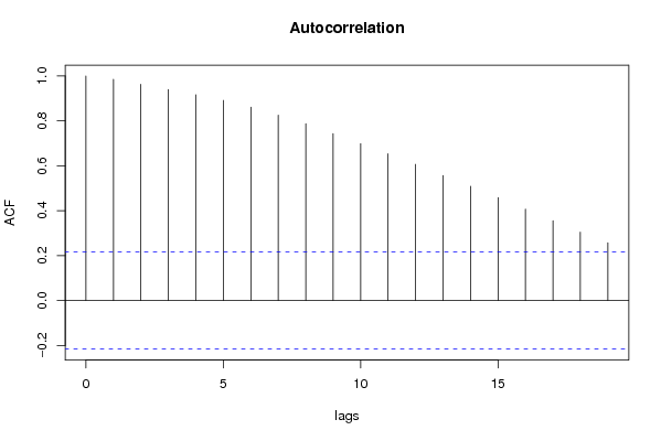
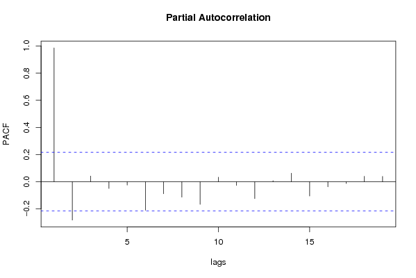
Title produced by software

(Partial) Autocorrelation Function

Date of computation

Wed, 03 Dec 2008 06:05:59 -0700

Cite this page as follows

Statistical Computations at FreeStatistics.org, Office for Research Development and Education, URL https://freestatistics.org/blog/index.php?v=date/2008/Dec/03/t1228309644pmqgb408jefp19s.htm/, Retrieved Fri, 17 May 2024 17:27:51 +0000

Statistical Computations at FreeStatistics.org, Office for Research Development and Education, URL https://freestatistics.org/blog/index.php?pk=28682, Retrieved Fri, 17 May 2024 17:27:51 +0000

QR Codes:

Paste this QR Code to cite your computation.

Original text written by user:

IsPrivate?

No (this computation is public)

User-defined keywords

Estimated Impact

222

Family? (F = Feedback message, R = changed R code, M = changed R Module, P = changed Parameters, D = changed Data)

F       [(Partial) Autocorrelation Function] [paper bel20 autoc...] [2008-12-03 13:05:59] [b09437381d488816ab9f5cf07e347c02] [Current]
-   PD    [(Partial) Autocorrelation Function] [paper autocorrela...] [2008-12-03 14:02:03] [f58cc3b532da25682c394745f1a82535] 
-   P       [(Partial) Autocorrelation Function] [] [2008-12-07 15:14:25] [74be16979710d4c4e7c6647856088456] 
-   P       [(Partial) Autocorrelation Function] [] [2008-12-11 15:54:51] [74be16979710d4c4e7c6647856088456] 
-   PD    [(Partial) Autocorrelation Function] [paper variance re...] [2008-12-03 14:08:24] [f58cc3b532da25682c394745f1a82535] 
F RM        [Variance Reduction Matrix] [paper variance re...] [2008-12-03 14:36:31] [f58cc3b532da25682c394745f1a82535] 
- RM        [Spectral Analysis] [paper spectral an...] [2008-12-03 14:40:03] [f58cc3b532da25682c394745f1a82535] 
-   P         [Spectral Analysis] [] [2008-12-07 15:17:33] [74be16979710d4c4e7c6647856088456] 
F RMPD          [(Partial) Autocorrelation Function] [] [2008-12-09 17:15:40] [300682cb535653f8775e6b312a464dab] 
F RMPD          [ARIMA Backward Selection] [] [2008-12-09 17:28:14] [300682cb535653f8775e6b312a464dab] 
- RMP           [(Partial) Autocorrelation Function] [] [2008-12-09 17:35:17] [300682cb535653f8775e6b312a464dab] 
F RMP           [ARIMA Backward Selection] [] [2008-12-09 18:26:36] [300682cb535653f8775e6b312a464dab] 
-   P             [ARIMA Backward Selection] [] [2008-12-13 14:37:56] [74be16979710d4c4e7c6647856088456] 
-   P             [ARIMA Backward Selection] [] [2008-12-14 15:26:26] [74be16979710d4c4e7c6647856088456] 
-   P               [ARIMA Backward Selection] [] [2008-12-15 18:05:04] [74be16979710d4c4e7c6647856088456] 
-   P                 [ARIMA Backward Selection] [] [2008-12-16 16:31:14] [74be16979710d4c4e7c6647856088456] 
F RMP                   [ARIMA Forecasting] [] [2008-12-16 17:13:10] [74be16979710d4c4e7c6647856088456] 
-   P         [Spectral Analysis] [] [2008-12-14 13:18:06] [74be16979710d4c4e7c6647856088456] 
-   PD    [(Partial) Autocorrelation Function] [] [2008-12-11 15:11:23] [74be16979710d4c4e7c6647856088456] 

Feedback Forum

2008-12-13 14:13:43 [Ken Wright] [reply] 
correct, om aan te tonen dat er geen seizoenaliteit is, kon ik nog zeggen dat er geen verhoogde waarden waren op lag 12;24;36,...

Post a new message

Dataseries X:

Download CSV

Histogram

Boxplots

Summary of computational transaction
Raw Input	view raw input (R code)
Raw Output	view raw output of R engine
Computing time	2 seconds
R Server	'Sir Ronald Aylmer Fisher' @ 193.190.124.24

\begin{tabular}{lllllllll}
\hline
Summary of computational transaction \tabularnewline
Raw Input & view raw input (R code)  \tabularnewline
Raw Output & view raw output of R engine  \tabularnewline
Computing time & 2 seconds \tabularnewline
R Server & 'Sir Ronald Aylmer Fisher' @ 193.190.124.24 \tabularnewline
\hline
\end{tabular}
%Source: https://freestatistics.org/blog/index.php?pk=28682&T=0

[TABLE]
[ROW][C]Summary of computational transaction[/C][/ROW]
[ROW][C]Raw Input[/C][C]view raw input (R code) [/C][/ROW]
[ROW][C]Raw Output[/C][C]view raw output of R engine [/C][/ROW]
[ROW][C]Computing time[/C][C]2 seconds[/C][/ROW]
[ROW][C]R Server[/C][C]'Sir Ronald Aylmer Fisher' @ 193.190.124.24[/C][/ROW]
[/TABLE]
Source: https://freestatistics.org/blog/index.php?pk=28682&T=0

Globally Unique Identifier (entire table): ba.freestatistics.org/blog/index.php?pk=28682&T=0

As an alternative you can also use a QR Code:

The GUIDs for individual cells are displayed in the table below:

Summary of computational transaction
Raw Input	view raw input (R code)
Raw Output	view raw output of R engine
Computing time	2 seconds
R Server	'Sir Ronald Aylmer Fisher' @ 193.190.124.24

Autocorrelation Function
Time lag k	ACF(k)	T-STAT	P-value
1	0.985514	8.9242	0
2	0.963104	8.7213	0
3	0.939966	8.5118	0
4	0.916037	8.2951	0
5	0.8913	8.0711	0
6	0.861056	7.7972	0
7	0.826002	7.4798	0
8	0.787081	7.1273	0
9	0.743034	6.7285	0
10	0.698582	6.3259	0
11	0.654089	5.923	0
12	0.606272	5.49	0
13	0.557113	5.0449	1e-06
14	0.508606	4.6056	7e-06
15	0.458472	4.1516	4e-05
16	0.407157	3.687	0.000203
17	0.354939	3.2141	0.000936
18	0.304412	2.7566	0.003599
19	0.25716	2.3287	0.011169

\begin{tabular}{lllllllll}
\hline
Autocorrelation Function \tabularnewline
Time lag k & ACF(k) & T-STAT & P-value \tabularnewline
1 & 0.985514 & 8.9242 & 0 \tabularnewline
2 & 0.963104 & 8.7213 & 0 \tabularnewline
3 & 0.939966 & 8.5118 & 0 \tabularnewline
4 & 0.916037 & 8.2951 & 0 \tabularnewline
5 & 0.8913 & 8.0711 & 0 \tabularnewline
6 & 0.861056 & 7.7972 & 0 \tabularnewline
7 & 0.826002 & 7.4798 & 0 \tabularnewline
8 & 0.787081 & 7.1273 & 0 \tabularnewline
9 & 0.743034 & 6.7285 & 0 \tabularnewline
10 & 0.698582 & 6.3259 & 0 \tabularnewline
11 & 0.654089 & 5.923 & 0 \tabularnewline
12 & 0.606272 & 5.49 & 0 \tabularnewline
13 & 0.557113 & 5.0449 & 1e-06 \tabularnewline
14 & 0.508606 & 4.6056 & 7e-06 \tabularnewline
15 & 0.458472 & 4.1516 & 4e-05 \tabularnewline
16 & 0.407157 & 3.687 & 0.000203 \tabularnewline
17 & 0.354939 & 3.2141 & 0.000936 \tabularnewline
18 & 0.304412 & 2.7566 & 0.003599 \tabularnewline
19 & 0.25716 & 2.3287 & 0.011169 \tabularnewline
\hline
\end{tabular}
%Source: https://freestatistics.org/blog/index.php?pk=28682&T=1

[TABLE]
[ROW][C]Autocorrelation Function[/C][/ROW]
[ROW][C]Time lag k[/C][C]ACF(k)[/C][C]T-STAT[/C][C]P-value[/C][/ROW]
[ROW][C]1[/C][C]0.985514[/C][C]8.9242[/C][C]0[/C][/ROW]
[ROW][C]2[/C][C]0.963104[/C][C]8.7213[/C][C]0[/C][/ROW]
[ROW][C]3[/C][C]0.939966[/C][C]8.5118[/C][C]0[/C][/ROW]
[ROW][C]4[/C][C]0.916037[/C][C]8.2951[/C][C]0[/C][/ROW]
[ROW][C]5[/C][C]0.8913[/C][C]8.0711[/C][C]0[/C][/ROW]
[ROW][C]6[/C][C]0.861056[/C][C]7.7972[/C][C]0[/C][/ROW]
[ROW][C]7[/C][C]0.826002[/C][C]7.4798[/C][C]0[/C][/ROW]
[ROW][C]8[/C][C]0.787081[/C][C]7.1273[/C][C]0[/C][/ROW]
[ROW][C]9[/C][C]0.743034[/C][C]6.7285[/C][C]0[/C][/ROW]
[ROW][C]10[/C][C]0.698582[/C][C]6.3259[/C][C]0[/C][/ROW]
[ROW][C]11[/C][C]0.654089[/C][C]5.923[/C][C]0[/C][/ROW]
[ROW][C]12[/C][C]0.606272[/C][C]5.49[/C][C]0[/C][/ROW]
[ROW][C]13[/C][C]0.557113[/C][C]5.0449[/C][C]1e-06[/C][/ROW]
[ROW][C]14[/C][C]0.508606[/C][C]4.6056[/C][C]7e-06[/C][/ROW]
[ROW][C]15[/C][C]0.458472[/C][C]4.1516[/C][C]4e-05[/C][/ROW]
[ROW][C]16[/C][C]0.407157[/C][C]3.687[/C][C]0.000203[/C][/ROW]
[ROW][C]17[/C][C]0.354939[/C][C]3.2141[/C][C]0.000936[/C][/ROW]
[ROW][C]18[/C][C]0.304412[/C][C]2.7566[/C][C]0.003599[/C][/ROW]
[ROW][C]19[/C][C]0.25716[/C][C]2.3287[/C][C]0.011169[/C][/ROW]
[/TABLE]
Source: https://freestatistics.org/blog/index.php?pk=28682&T=1

Globally Unique Identifier (entire table): ba.freestatistics.org/blog/index.php?pk=28682&T=1

As an alternative you can also use a QR Code:

The GUIDs for individual cells are displayed in the table below:

Autocorrelation Function
Time lag k	ACF(k)	T-STAT	P-value
1	0.985514	8.9242	0
2	0.963104	8.7213	0
3	0.939966	8.5118	0
4	0.916037	8.2951	0
5	0.8913	8.0711	0
6	0.861056	7.7972	0
7	0.826002	7.4798	0
8	0.787081	7.1273	0
9	0.743034	6.7285	0
10	0.698582	6.3259	0
11	0.654089	5.923	0
12	0.606272	5.49	0
13	0.557113	5.0449	1e-06
14	0.508606	4.6056	7e-06
15	0.458472	4.1516	4e-05
16	0.407157	3.687	0.000203
17	0.354939	3.2141	0.000936
18	0.304412	2.7566	0.003599
19	0.25716	2.3287	0.011169

Partial Autocorrelation Function
Time lag k	PACF(k)	T-STAT	P-value
1	0.985514	8.9242	0
2	-0.282797	-2.5608	0.006137
3	0.041476	0.3756	0.354098
4	-0.049941	-0.4522	0.326147
5	-0.025216	-0.2283	0.409976
6	-0.210901	-1.9098	0.029828
7	-0.089192	-0.8077	0.210809
8	-0.113876	-1.0312	0.152742
9	-0.166721	-1.5097	0.067479
10	0.033476	0.3031	0.381277
11	-0.027371	-0.2479	0.402433
12	-0.124806	-1.1302	0.13085
13	0.007677	0.0695	0.472375
14	0.06242	0.5652	0.286729
15	-0.105331	-0.9538	0.171492
16	-0.037213	-0.337	0.368497
17	-0.01327	-0.1202	0.452321
18	0.039046	0.3536	0.362283
19	0.038731	0.3507	0.363346

\begin{tabular}{lllllllll}
\hline
Partial Autocorrelation Function \tabularnewline
Time lag k & PACF(k) & T-STAT & P-value \tabularnewline
1 & 0.985514 & 8.9242 & 0 \tabularnewline
2 & -0.282797 & -2.5608 & 0.006137 \tabularnewline
3 & 0.041476 & 0.3756 & 0.354098 \tabularnewline
4 & -0.049941 & -0.4522 & 0.326147 \tabularnewline
5 & -0.025216 & -0.2283 & 0.409976 \tabularnewline
6 & -0.210901 & -1.9098 & 0.029828 \tabularnewline
7 & -0.089192 & -0.8077 & 0.210809 \tabularnewline
8 & -0.113876 & -1.0312 & 0.152742 \tabularnewline
9 & -0.166721 & -1.5097 & 0.067479 \tabularnewline
10 & 0.033476 & 0.3031 & 0.381277 \tabularnewline
11 & -0.027371 & -0.2479 & 0.402433 \tabularnewline
12 & -0.124806 & -1.1302 & 0.13085 \tabularnewline
13 & 0.007677 & 0.0695 & 0.472375 \tabularnewline
14 & 0.06242 & 0.5652 & 0.286729 \tabularnewline
15 & -0.105331 & -0.9538 & 0.171492 \tabularnewline
16 & -0.037213 & -0.337 & 0.368497 \tabularnewline
17 & -0.01327 & -0.1202 & 0.452321 \tabularnewline
18 & 0.039046 & 0.3536 & 0.362283 \tabularnewline
19 & 0.038731 & 0.3507 & 0.363346 \tabularnewline
\hline
\end{tabular}
%Source: https://freestatistics.org/blog/index.php?pk=28682&T=2

[TABLE]
[ROW][C]Partial Autocorrelation Function[/C][/ROW]
[ROW][C]Time lag k[/C][C]PACF(k)[/C][C]T-STAT[/C][C]P-value[/C][/ROW]
[ROW][C]1[/C][C]0.985514[/C][C]8.9242[/C][C]0[/C][/ROW]
[ROW][C]2[/C][C]-0.282797[/C][C]-2.5608[/C][C]0.006137[/C][/ROW]
[ROW][C]3[/C][C]0.041476[/C][C]0.3756[/C][C]0.354098[/C][/ROW]
[ROW][C]4[/C][C]-0.049941[/C][C]-0.4522[/C][C]0.326147[/C][/ROW]
[ROW][C]5[/C][C]-0.025216[/C][C]-0.2283[/C][C]0.409976[/C][/ROW]
[ROW][C]6[/C][C]-0.210901[/C][C]-1.9098[/C][C]0.029828[/C][/ROW]
[ROW][C]7[/C][C]-0.089192[/C][C]-0.8077[/C][C]0.210809[/C][/ROW]
[ROW][C]8[/C][C]-0.113876[/C][C]-1.0312[/C][C]0.152742[/C][/ROW]
[ROW][C]9[/C][C]-0.166721[/C][C]-1.5097[/C][C]0.067479[/C][/ROW]
[ROW][C]10[/C][C]0.033476[/C][C]0.3031[/C][C]0.381277[/C][/ROW]
[ROW][C]11[/C][C]-0.027371[/C][C]-0.2479[/C][C]0.402433[/C][/ROW]
[ROW][C]12[/C][C]-0.124806[/C][C]-1.1302[/C][C]0.13085[/C][/ROW]
[ROW][C]13[/C][C]0.007677[/C][C]0.0695[/C][C]0.472375[/C][/ROW]
[ROW][C]14[/C][C]0.06242[/C][C]0.5652[/C][C]0.286729[/C][/ROW]
[ROW][C]15[/C][C]-0.105331[/C][C]-0.9538[/C][C]0.171492[/C][/ROW]
[ROW][C]16[/C][C]-0.037213[/C][C]-0.337[/C][C]0.368497[/C][/ROW]
[ROW][C]17[/C][C]-0.01327[/C][C]-0.1202[/C][C]0.452321[/C][/ROW]
[ROW][C]18[/C][C]0.039046[/C][C]0.3536[/C][C]0.362283[/C][/ROW]
[ROW][C]19[/C][C]0.038731[/C][C]0.3507[/C][C]0.363346[/C][/ROW]
[/TABLE]
Source: https://freestatistics.org/blog/index.php?pk=28682&T=2

Globally Unique Identifier (entire table): ba.freestatistics.org/blog/index.php?pk=28682&T=2

As an alternative you can also use a QR Code:

The GUIDs for individual cells are displayed in the table below:

Partial Autocorrelation Function
Time lag k	PACF(k)	T-STAT	P-value
1	0.985514	8.9242	0
2	-0.282797	-2.5608	0.006137
3	0.041476	0.3756	0.354098
4	-0.049941	-0.4522	0.326147
5	-0.025216	-0.2283	0.409976
6	-0.210901	-1.9098	0.029828
7	-0.089192	-0.8077	0.210809
8	-0.113876	-1.0312	0.152742
9	-0.166721	-1.5097	0.067479
10	0.033476	0.3031	0.381277
11	-0.027371	-0.2479	0.402433
12	-0.124806	-1.1302	0.13085
13	0.007677	0.0695	0.472375
14	0.06242	0.5652	0.286729
15	-0.105331	-0.9538	0.171492
16	-0.037213	-0.337	0.368497
17	-0.01327	-0.1202	0.452321
18	0.039046	0.3536	0.362283
19	0.038731	0.3507	0.363346

Figure 1

PNG link

Postscript link

PDF link

Figure 2

PNG link

Postscript link

PDF link

Parameters (Session):

par1 = Default ; par2 = 1 ; par3 = 0 ; par4 = 0 ; par5 = 12 ;

Parameters (R input):

par1 = Default ; par2 = 1 ; par3 = 0 ; par4 = 0 ; par5 = 12 ;

R code (references can be found in the software module):

if (par1 == 'Default') {
par1 = 10*log10(length(x))
} else {
par1 <- as.numeric(par1)
}
par2 <- as.numeric(par2)
par3 <- as.numeric(par3)
par4 <- as.numeric(par4)
par5 <- as.numeric(par5)
if (par2 == 0) {
x <- log(x)
} else {
x <- (x ^ par2 - 1) / par2
}
if (par3 > 0) x <- diff(x,lag=1,difference=par3)
if (par4 > 0) x <- diff(x,lag=par5,difference=par4)
bitmap(file='pic1.png')
racf <- acf(x,par1,main='Autocorrelation',xlab='lags',ylab='ACF')
dev.off()
bitmap(file='pic2.png')
rpacf <- pacf(x,par1,main='Partial Autocorrelation',xlab='lags',ylab='PACF')
dev.off()
(myacf <- c(racf$acf))
(mypacf <- c(rpacf$acf))
lengthx <- length(x)
sqrtn <- sqrt(lengthx)
load(file='createtable')
a<-table.start()
a<-table.row.start(a)
a<-table.element(a,'Autocorrelation Function',4,TRUE)
a<-table.row.end(a)
a<-table.row.start(a)
a<-table.element(a,'Time lag k',header=TRUE)
a<-table.element(a,hyperlink('basics.htm','ACF(k)','click here for more information about the Autocorrelation Function'),header=TRUE)
a<-table.element(a,'T-STAT',header=TRUE)
a<-table.element(a,'P-value',header=TRUE)
a<-table.row.end(a)
for (i in 2:(par1+1)) {
a<-table.row.start(a)
a<-table.element(a,i-1,header=TRUE)
a<-table.element(a,round(myacf[i],6))
mytstat <- myacf[i]*sqrtn
a<-table.element(a,round(mytstat,4))
a<-table.element(a,round(1-pt(abs(mytstat),lengthx),6))
a<-table.row.end(a)
}
a<-table.end(a)
table.save(a,file='mytable.tab')
a<-table.start()
a<-table.row.start(a)
a<-table.element(a,'Partial Autocorrelation Function',4,TRUE)
a<-table.row.end(a)
a<-table.row.start(a)
a<-table.element(a,'Time lag k',header=TRUE)
a<-table.element(a,hyperlink('basics.htm','PACF(k)','click here for more information about the Partial Autocorrelation Function'),header=TRUE)
a<-table.element(a,'T-STAT',header=TRUE)
a<-table.element(a,'P-value',header=TRUE)
a<-table.row.end(a)
for (i in 1:par1) {
a<-table.row.start(a)
a<-table.element(a,i,header=TRUE)
a<-table.element(a,round(mypacf[i],6))
mytstat <- mypacf[i]*sqrtn
a<-table.element(a,round(mytstat,4))
a<-table.element(a,round(1-pt(abs(mytstat),lengthx),6))
a<-table.row.end(a)
}
a<-table.end(a)
table.save(a,file='mytable1.tab')

Free Statistics

Description of Statistical Computation

Tree of Dependent Computations

Dataset

Tables (Output of Computation)

Figures (Output of Computation)

Input Parameters & R Code