Repository of Reproducible Computations

Free Statistics

of Irreproducible Research!

Author's title

Author

*Unverified author*

R Software Module

rwasp_smp.wasp

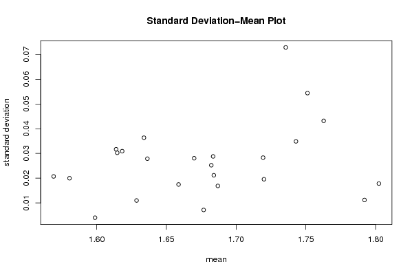
Title produced by software

Standard Deviation-Mean Plot

Date of computation

Wed, 03 Dec 2008 01:52:51 -0700

Cite this page as follows

Statistical Computations at FreeStatistics.org, Office for Research Development and Education, URL https://freestatistics.org/blog/index.php?v=date/2008/Dec/03/t12282944082bd6tia1umboztn.htm/, Retrieved Fri, 17 May 2024 16:56:02 +0000

Statistical Computations at FreeStatistics.org, Office for Research Development and Education, URL https://freestatistics.org/blog/index.php?pk=28579, Retrieved Fri, 17 May 2024 16:56:02 +0000

QR Codes:

Paste this QR Code to cite your computation.

Original text written by user:

IsPrivate?

No (this computation is public)

User-defined keywords

Estimated Impact

178

Family? (F = Feedback message, R = changed R code, M = changed R Module, P = changed Parameters, D = changed Data)

F       [Standard Deviation-Mean Plot] [] [2008-12-03 08:52:51] [ee5aee65e0c44ac54c8097a6e28e37f4] [Current]

Feedback Forum

2008-12-08 13:48:32 [Li Tang Hu] [reply] 
Ook hier is de lambdawaarde onbruikbaar omdat de pwaarden veel te groot zijn.

Post a new message

Dataseries X:

Download CSV

Histogram

Boxplots

Summary of computational transaction
Raw Input	view raw input (R code)
Raw Output	view raw output of R engine
Computing time	2 seconds
R Server	'George Udny Yule' @ 72.249.76.132

\begin{tabular}{lllllllll}
\hline
Summary of computational transaction \tabularnewline
Raw Input & view raw input (R code)  \tabularnewline
Raw Output & view raw output of R engine  \tabularnewline
Computing time & 2 seconds \tabularnewline
R Server & 'George Udny Yule' @ 72.249.76.132 \tabularnewline
\hline
\end{tabular}
%Source: https://freestatistics.org/blog/index.php?pk=28579&T=0

[TABLE]
[ROW][C]Summary of computational transaction[/C][/ROW]
[ROW][C]Raw Input[/C][C]view raw input (R code) [/C][/ROW]
[ROW][C]Raw Output[/C][C]view raw output of R engine [/C][/ROW]
[ROW][C]Computing time[/C][C]2 seconds[/C][/ROW]
[ROW][C]R Server[/C][C]'George Udny Yule' @ 72.249.76.132[/C][/ROW]
[/TABLE]
Source: https://freestatistics.org/blog/index.php?pk=28579&T=0

Globally Unique Identifier (entire table): ba.freestatistics.org/blog/index.php?pk=28579&T=0

As an alternative you can also use a QR Code:

The GUIDs for individual cells are displayed in the table below:

Summary of computational transaction
Raw Input	view raw input (R code)
Raw Output	view raw output of R engine
Computing time	2 seconds
R Server	'George Udny Yule' @ 72.249.76.132

Standard Deviation-Mean Plot
Section	Mean	Standard Deviation	Range
1	1.5692	0.0207173035568499	0.0457000000000001
2	1.5806	0.0199831595766702	0.0403
3	1.61835	0.0309376254206212	0.0673000000000001
4	1.75115	0.0543948833378042	0.1181
5	1.683525	0.0288109209617927	0.07
6	1.762775	0.0431944730260713	0.0864
7	1.682225	0.0252466994542521	0.0557000000000001
8	1.73555	0.0728853208815054	0.1383
9	1.792025	0.0112004092187147	0.0245000000000002
10	1.802325	0.0178301944278051	0.0405
11	1.7429	0.0348973733491027	0.0752
12	1.669925	0.0280725696484428	0.0630000000000002
13	1.62865	0.0109865068758606	0.0231999999999999
14	1.71995	0.0195798365672444	0.0449999999999999
15	1.71935	0.0283184863060628	0.0594999999999999
16	1.684025	0.0211903083192922	0.0476999999999999
17	1.6148	0.0302649412136662	0.0696000000000001
18	1.598875	0.00403515798947206	0.00930000000000009
19	1.6364	0.0278907392037811	0.0559999999999998
20	1.6869	0.0168821404646053	0.0388999999999999
21	1.67675	0.00717333023543918	0.0154999999999998
22	1.65875	0.0174694972261177	0.0372000000000001
23	1.613975	0.0317021949818411	0.0633000000000001
24	1.63395	0.0363726545635591	0.0865999999999998

\begin{tabular}{lllllllll}
\hline
Standard Deviation-Mean Plot \tabularnewline
Section & Mean & Standard Deviation & Range \tabularnewline
1 & 1.5692 & 0.0207173035568499 & 0.0457000000000001 \tabularnewline
2 & 1.5806 & 0.0199831595766702 & 0.0403 \tabularnewline
3 & 1.61835 & 0.0309376254206212 & 0.0673000000000001 \tabularnewline
4 & 1.75115 & 0.0543948833378042 & 0.1181 \tabularnewline
5 & 1.683525 & 0.0288109209617927 & 0.07 \tabularnewline
6 & 1.762775 & 0.0431944730260713 & 0.0864 \tabularnewline
7 & 1.682225 & 0.0252466994542521 & 0.0557000000000001 \tabularnewline
8 & 1.73555 & 0.0728853208815054 & 0.1383 \tabularnewline
9 & 1.792025 & 0.0112004092187147 & 0.0245000000000002 \tabularnewline
10 & 1.802325 & 0.0178301944278051 & 0.0405 \tabularnewline
11 & 1.7429 & 0.0348973733491027 & 0.0752 \tabularnewline
12 & 1.669925 & 0.0280725696484428 & 0.0630000000000002 \tabularnewline
13 & 1.62865 & 0.0109865068758606 & 0.0231999999999999 \tabularnewline
14 & 1.71995 & 0.0195798365672444 & 0.0449999999999999 \tabularnewline
15 & 1.71935 & 0.0283184863060628 & 0.0594999999999999 \tabularnewline
16 & 1.684025 & 0.0211903083192922 & 0.0476999999999999 \tabularnewline
17 & 1.6148 & 0.0302649412136662 & 0.0696000000000001 \tabularnewline
18 & 1.598875 & 0.00403515798947206 & 0.00930000000000009 \tabularnewline
19 & 1.6364 & 0.0278907392037811 & 0.0559999999999998 \tabularnewline
20 & 1.6869 & 0.0168821404646053 & 0.0388999999999999 \tabularnewline
21 & 1.67675 & 0.00717333023543918 & 0.0154999999999998 \tabularnewline
22 & 1.65875 & 0.0174694972261177 & 0.0372000000000001 \tabularnewline
23 & 1.613975 & 0.0317021949818411 & 0.0633000000000001 \tabularnewline
24 & 1.63395 & 0.0363726545635591 & 0.0865999999999998 \tabularnewline
\hline
\end{tabular}
%Source: https://freestatistics.org/blog/index.php?pk=28579&T=1

[TABLE]
[ROW][C]Standard Deviation-Mean Plot[/C][/ROW]
[ROW][C]Section[/C][C]Mean[/C][C]Standard Deviation[/C][C]Range[/C][/ROW]
[ROW][C]1[/C][C]1.5692[/C][C]0.0207173035568499[/C][C]0.0457000000000001[/C][/ROW]
[ROW][C]2[/C][C]1.5806[/C][C]0.0199831595766702[/C][C]0.0403[/C][/ROW]
[ROW][C]3[/C][C]1.61835[/C][C]0.0309376254206212[/C][C]0.0673000000000001[/C][/ROW]
[ROW][C]4[/C][C]1.75115[/C][C]0.0543948833378042[/C][C]0.1181[/C][/ROW]
[ROW][C]5[/C][C]1.683525[/C][C]0.0288109209617927[/C][C]0.07[/C][/ROW]
[ROW][C]6[/C][C]1.762775[/C][C]0.0431944730260713[/C][C]0.0864[/C][/ROW]
[ROW][C]7[/C][C]1.682225[/C][C]0.0252466994542521[/C][C]0.0557000000000001[/C][/ROW]
[ROW][C]8[/C][C]1.73555[/C][C]0.0728853208815054[/C][C]0.1383[/C][/ROW]
[ROW][C]9[/C][C]1.792025[/C][C]0.0112004092187147[/C][C]0.0245000000000002[/C][/ROW]
[ROW][C]10[/C][C]1.802325[/C][C]0.0178301944278051[/C][C]0.0405[/C][/ROW]
[ROW][C]11[/C][C]1.7429[/C][C]0.0348973733491027[/C][C]0.0752[/C][/ROW]
[ROW][C]12[/C][C]1.669925[/C][C]0.0280725696484428[/C][C]0.0630000000000002[/C][/ROW]
[ROW][C]13[/C][C]1.62865[/C][C]0.0109865068758606[/C][C]0.0231999999999999[/C][/ROW]
[ROW][C]14[/C][C]1.71995[/C][C]0.0195798365672444[/C][C]0.0449999999999999[/C][/ROW]
[ROW][C]15[/C][C]1.71935[/C][C]0.0283184863060628[/C][C]0.0594999999999999[/C][/ROW]
[ROW][C]16[/C][C]1.684025[/C][C]0.0211903083192922[/C][C]0.0476999999999999[/C][/ROW]
[ROW][C]17[/C][C]1.6148[/C][C]0.0302649412136662[/C][C]0.0696000000000001[/C][/ROW]
[ROW][C]18[/C][C]1.598875[/C][C]0.00403515798947206[/C][C]0.00930000000000009[/C][/ROW]
[ROW][C]19[/C][C]1.6364[/C][C]0.0278907392037811[/C][C]0.0559999999999998[/C][/ROW]
[ROW][C]20[/C][C]1.6869[/C][C]0.0168821404646053[/C][C]0.0388999999999999[/C][/ROW]
[ROW][C]21[/C][C]1.67675[/C][C]0.00717333023543918[/C][C]0.0154999999999998[/C][/ROW]
[ROW][C]22[/C][C]1.65875[/C][C]0.0174694972261177[/C][C]0.0372000000000001[/C][/ROW]
[ROW][C]23[/C][C]1.613975[/C][C]0.0317021949818411[/C][C]0.0633000000000001[/C][/ROW]
[ROW][C]24[/C][C]1.63395[/C][C]0.0363726545635591[/C][C]0.0865999999999998[/C][/ROW]
[/TABLE]
Source: https://freestatistics.org/blog/index.php?pk=28579&T=1

Globally Unique Identifier (entire table): ba.freestatistics.org/blog/index.php?pk=28579&T=1

As an alternative you can also use a QR Code:

The GUIDs for individual cells are displayed in the table below:

Standard Deviation-Mean Plot
Section	Mean	Standard Deviation	Range
1	1.5692	0.0207173035568499	0.0457000000000001
2	1.5806	0.0199831595766702	0.0403
3	1.61835	0.0309376254206212	0.0673000000000001
4	1.75115	0.0543948833378042	0.1181
5	1.683525	0.0288109209617927	0.07
6	1.762775	0.0431944730260713	0.0864
7	1.682225	0.0252466994542521	0.0557000000000001
8	1.73555	0.0728853208815054	0.1383
9	1.792025	0.0112004092187147	0.0245000000000002
10	1.802325	0.0178301944278051	0.0405
11	1.7429	0.0348973733491027	0.0752
12	1.669925	0.0280725696484428	0.0630000000000002
13	1.62865	0.0109865068758606	0.0231999999999999
14	1.71995	0.0195798365672444	0.0449999999999999
15	1.71935	0.0283184863060628	0.0594999999999999
16	1.684025	0.0211903083192922	0.0476999999999999
17	1.6148	0.0302649412136662	0.0696000000000001
18	1.598875	0.00403515798947206	0.00930000000000009
19	1.6364	0.0278907392037811	0.0559999999999998
20	1.6869	0.0168821404646053	0.0388999999999999
21	1.67675	0.00717333023543918	0.0154999999999998
22	1.65875	0.0174694972261177	0.0372000000000001
23	1.613975	0.0317021949818411	0.0633000000000001
24	1.63395	0.0363726545635591	0.0865999999999998

Regression: S.E.(k) = alpha + beta * Mean(k)
alpha	-0.07933676096463
beta	0.0631876345287307
S.D.	0.0472717998629565
T-STAT	1.33668772316508
p-value	0.194984635923570

\begin{tabular}{lllllllll}
\hline
Regression: S.E.(k) = alpha + beta * Mean(k) \tabularnewline
alpha & -0.07933676096463 \tabularnewline
beta & 0.0631876345287307 \tabularnewline
S.D. & 0.0472717998629565 \tabularnewline
T-STAT & 1.33668772316508 \tabularnewline
p-value & 0.194984635923570 \tabularnewline
\hline
\end{tabular}
%Source: https://freestatistics.org/blog/index.php?pk=28579&T=2

[TABLE]
[ROW][C]Regression: S.E.(k) = alpha + beta * Mean(k)[/C][/ROW]
[ROW][C]alpha[/C][C]-0.07933676096463[/C][/ROW]
[ROW][C]beta[/C][C]0.0631876345287307[/C][/ROW]
[ROW][C]S.D.[/C][C]0.0472717998629565[/C][/ROW]
[ROW][C]T-STAT[/C][C]1.33668772316508[/C][/ROW]
[ROW][C]p-value[/C][C]0.194984635923570[/C][/ROW]
[/TABLE]
Source: https://freestatistics.org/blog/index.php?pk=28579&T=2

Globally Unique Identifier (entire table): ba.freestatistics.org/blog/index.php?pk=28579&T=2

As an alternative you can also use a QR Code:

The GUIDs for individual cells are displayed in the table below:

Regression: S.E.(k) = alpha + beta * Mean(k)
alpha	-0.07933676096463
beta	0.0631876345287307
S.D.	0.0472717998629565
T-STAT	1.33668772316508
p-value	0.194984635923570

Regression: ln S.E.(k) = alpha + beta * ln Mean(k)
alpha	-5.73882044141911
beta	3.77722844612018
S.D.	3.35208505653102
T-STAT	1.12682953517568
p-value	0.271955806773729
Lambda	-2.77722844612018

\begin{tabular}{lllllllll}
\hline
Regression: ln S.E.(k) = alpha + beta * ln Mean(k) \tabularnewline
alpha & -5.73882044141911 \tabularnewline
beta & 3.77722844612018 \tabularnewline
S.D. & 3.35208505653102 \tabularnewline
T-STAT & 1.12682953517568 \tabularnewline
p-value & 0.271955806773729 \tabularnewline
Lambda & -2.77722844612018 \tabularnewline
\hline
\end{tabular}
%Source: https://freestatistics.org/blog/index.php?pk=28579&T=3

[TABLE]
[ROW][C]Regression: ln S.E.(k) = alpha + beta * ln Mean(k)[/C][/ROW]
[ROW][C]alpha[/C][C]-5.73882044141911[/C][/ROW]
[ROW][C]beta[/C][C]3.77722844612018[/C][/ROW]
[ROW][C]S.D.[/C][C]3.35208505653102[/C][/ROW]
[ROW][C]T-STAT[/C][C]1.12682953517568[/C][/ROW]
[ROW][C]p-value[/C][C]0.271955806773729[/C][/ROW]
[ROW][C]Lambda[/C][C]-2.77722844612018[/C][/ROW]
[/TABLE]
Source: https://freestatistics.org/blog/index.php?pk=28579&T=3

Globally Unique Identifier (entire table): ba.freestatistics.org/blog/index.php?pk=28579&T=3

As an alternative you can also use a QR Code:

The GUIDs for individual cells are displayed in the table below:

Regression: ln S.E.(k) = alpha + beta * ln Mean(k)
alpha	-5.73882044141911
beta	3.77722844612018
S.D.	3.35208505653102
T-STAT	1.12682953517568
p-value	0.271955806773729
Lambda	-2.77722844612018

Figure 1

PNG link

Postscript link

PDF link

Figure 2

PNG link

Postscript link

PDF link

Parameters (Session):

par1 = 4 ;

Parameters (R input):

par1 = 4 ;

R code (references can be found in the software module):

par1 <- as.numeric(par1)
(n <- length(x))
(np <- floor(n / par1))
arr <- array(NA,dim=c(par1,np))
j <- 0
k <- 1
for (i in 1:(np*par1))
{
j = j + 1
arr[j,k] <- x[i]
if (j == par1) {
j = 0
k=k+1
}
}
arr
arr.mean <- array(NA,dim=np)
arr.sd <- array(NA,dim=np)
arr.range <- array(NA,dim=np)
for (j in 1:np)
{
arr.mean[j] <- mean(arr[,j],na.rm=TRUE)
arr.sd[j] <- sd(arr[,j],na.rm=TRUE)
arr.range[j] <- max(arr[,j],na.rm=TRUE) - min(arr[,j],na.rm=TRUE)
}
arr.mean
arr.sd
arr.range
(lm1 <- lm(arr.sd~arr.mean))
(lnlm1 <- lm(log(arr.sd)~log(arr.mean)))
(lm2 <- lm(arr.range~arr.mean))
bitmap(file='test1.png')
plot(arr.mean,arr.sd,main='Standard Deviation-Mean Plot',xlab='mean',ylab='standard deviation')
dev.off()
bitmap(file='test2.png')
plot(arr.mean,arr.range,main='Range-Mean Plot',xlab='mean',ylab='range')
dev.off()
load(file='createtable')
a<-table.start()
a<-table.row.start(a)
a<-table.element(a,'Standard Deviation-Mean Plot',4,TRUE)
a<-table.row.end(a)
a<-table.row.start(a)
a<-table.element(a,'Section',header=TRUE)
a<-table.element(a,'Mean',header=TRUE)
a<-table.element(a,'Standard Deviation',header=TRUE)
a<-table.element(a,'Range',header=TRUE)
a<-table.row.end(a)
for (j in 1:np) {
a<-table.row.start(a)
a<-table.element(a,j,header=TRUE)
a<-table.element(a,arr.mean[j])
a<-table.element(a,arr.sd[j] )
a<-table.element(a,arr.range[j] )
a<-table.row.end(a)
}
a<-table.end(a)
table.save(a,file='mytable.tab')
a<-table.start()
a<-table.row.start(a)
a<-table.element(a,'Regression: S.E.(k) = alpha + beta * Mean(k)',2,TRUE)
a<-table.row.end(a)
a<-table.row.start(a)
a<-table.element(a,'alpha',header=TRUE)
a<-table.element(a,lm1$coefficients[[1]])
a<-table.row.end(a)
a<-table.row.start(a)
a<-table.element(a,'beta',header=TRUE)
a<-table.element(a,lm1$coefficients[[2]])
a<-table.row.end(a)
a<-table.row.start(a)
a<-table.element(a,'S.D.',header=TRUE)
a<-table.element(a,summary(lm1)$coefficients[2,2])
a<-table.row.end(a)
a<-table.row.start(a)
a<-table.element(a,'T-STAT',header=TRUE)
a<-table.element(a,summary(lm1)$coefficients[2,3])
a<-table.row.end(a)
a<-table.row.start(a)
a<-table.element(a,'p-value',header=TRUE)
a<-table.element(a,summary(lm1)$coefficients[2,4])
a<-table.row.end(a)
a<-table.end(a)
table.save(a,file='mytable1.tab')
a<-table.start()
a<-table.row.start(a)
a<-table.element(a,'Regression: ln S.E.(k) = alpha + beta * ln Mean(k)',2,TRUE)
a<-table.row.end(a)
a<-table.row.start(a)
a<-table.element(a,'alpha',header=TRUE)
a<-table.element(a,lnlm1$coefficients[[1]])
a<-table.row.end(a)
a<-table.row.start(a)
a<-table.element(a,'beta',header=TRUE)
a<-table.element(a,lnlm1$coefficients[[2]])
a<-table.row.end(a)
a<-table.row.start(a)
a<-table.element(a,'S.D.',header=TRUE)
a<-table.element(a,summary(lnlm1)$coefficients[2,2])
a<-table.row.end(a)
a<-table.row.start(a)
a<-table.element(a,'T-STAT',header=TRUE)
a<-table.element(a,summary(lnlm1)$coefficients[2,3])
a<-table.row.end(a)
a<-table.row.start(a)
a<-table.element(a,'p-value',header=TRUE)
a<-table.element(a,summary(lnlm1)$coefficients[2,4])
a<-table.row.end(a)
a<-table.row.start(a)
a<-table.element(a,'Lambda',header=TRUE)
a<-table.element(a,1-lnlm1$coefficients[[2]])
a<-table.row.end(a)
a<-table.end(a)
table.save(a,file='mytable2.tab')

Free Statistics

Description of Statistical Computation

Tree of Dependent Computations

Dataset

Tables (Output of Computation)

Figures (Output of Computation)

Input Parameters & R Code