Repository of Reproducible Computations

Free Statistics

of Irreproducible Research!

Author's title

Author

*Unverified author*

R Software Module

rwasp_autocorrelation.wasp

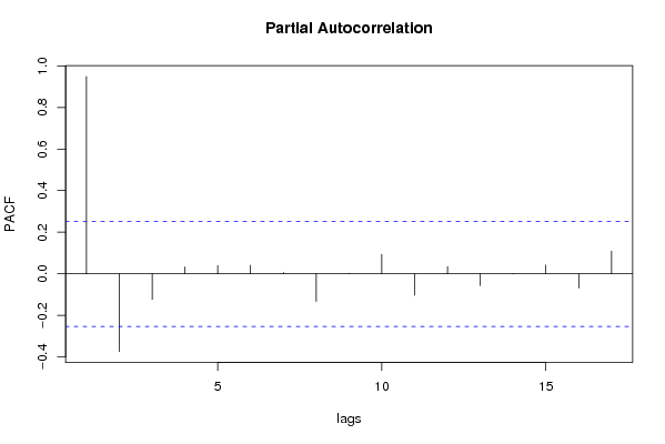
Title produced by software

(Partial) Autocorrelation Function

Date of computation

Wed, 03 Dec 2008 00:54:56 -0700

Cite this page as follows

Statistical Computations at FreeStatistics.org, Office for Research Development and Education, URL https://freestatistics.org/blog/index.php?v=date/2008/Dec/03/t12282909349lhs607fnofkh2v.htm/, Retrieved Fri, 17 May 2024 17:56:50 +0000

Statistical Computations at FreeStatistics.org, Office for Research Development and Education, URL https://freestatistics.org/blog/index.php?pk=28559, Retrieved Fri, 17 May 2024 17:56:50 +0000

QR Codes:

Paste this QR Code to cite your computation.

Original text written by user:

IsPrivate?

No (this computation is public)

User-defined keywords

Estimated Impact

233

Family? (F = Feedback message, R = changed R code, M = changed R Module, P = changed Parameters, D = changed Data)

F       [(Partial) Autocorrelation Function] [] [2008-12-03 07:54:56] [e02910eed3830f1815f587e12f46cbdb] [Current]
-   PD    [(Partial) Autocorrelation Function] [] [2008-12-06 11:50:22] [996314793dac993597edc1ca2281ff39] 

Feedback Forum

2008-12-06 11:53:21 [Angelique Van de Vijver] [reply] 
Student heeft in haar berekening number of time lags= default. 
Daarom heb ik de berekening opnieuw gemaakt met number of time lags = 36 http://www.freestatistics.org/blog/date/2008/Dec/06/t1228564245qeubkhbn6cjmeqz.htm 
We zien op de ACF nog altijd een langzaam dalend patroon => langetermijntrend. 
Dus hier moeten we ook niet-seizoenaal differentiëren.

Post a new message

Dataseries X:

Download CSV

Histogram

Boxplots

Summary of computational transaction
Raw Input	view raw input (R code)
Raw Output	view raw output of R engine
Computing time	1 seconds
R Server	'George Udny Yule' @ 72.249.76.132

\begin{tabular}{lllllllll}
\hline
Summary of computational transaction \tabularnewline
Raw Input & view raw input (R code)  \tabularnewline
Raw Output & view raw output of R engine  \tabularnewline
Computing time & 1 seconds \tabularnewline
R Server & 'George Udny Yule' @ 72.249.76.132 \tabularnewline
\hline
\end{tabular}
%Source: https://freestatistics.org/blog/index.php?pk=28559&T=0

[TABLE]
[ROW][C]Summary of computational transaction[/C][/ROW]
[ROW][C]Raw Input[/C][C]view raw input (R code) [/C][/ROW]
[ROW][C]Raw Output[/C][C]view raw output of R engine [/C][/ROW]
[ROW][C]Computing time[/C][C]1 seconds[/C][/ROW]
[ROW][C]R Server[/C][C]'George Udny Yule' @ 72.249.76.132[/C][/ROW]
[/TABLE]
Source: https://freestatistics.org/blog/index.php?pk=28559&T=0

Globally Unique Identifier (entire table): ba.freestatistics.org/blog/index.php?pk=28559&T=0

As an alternative you can also use a QR Code:

The GUIDs for individual cells are displayed in the table below:

Summary of computational transaction
Raw Input	view raw input (R code)
Raw Output	view raw output of R engine
Computing time	1 seconds
R Server	'George Udny Yule' @ 72.249.76.132

Autocorrelation Function
Time lag k	ACF(k)	T-STAT	P-value
1	0.948815	7.3495	0
2	0.862951	6.6844	0
3	0.759617	5.884	0
4	0.65712	5.09	2e-06
5	0.564901	4.3757	2.5e-05
6	0.488193	3.7815	0.000181
7	0.425673	3.2972	0.000822
8	0.363641	2.8168	0.003279
9	0.304688	2.3601	0.01077
10	0.256068	1.9835	0.025947
11	0.207573	1.6079	0.056559
12	0.16611	1.2867	0.101574
13	0.126243	0.9779	0.166031
14	0.091091	0.7056	0.241588
15	0.061918	0.4796	0.316623
16	0.03293	0.2551	0.399768
17	0.017392	0.1347	0.446643

\begin{tabular}{lllllllll}
\hline
Autocorrelation Function \tabularnewline
Time lag k & ACF(k) & T-STAT & P-value \tabularnewline
1 & 0.948815 & 7.3495 & 0 \tabularnewline
2 & 0.862951 & 6.6844 & 0 \tabularnewline
3 & 0.759617 & 5.884 & 0 \tabularnewline
4 & 0.65712 & 5.09 & 2e-06 \tabularnewline
5 & 0.564901 & 4.3757 & 2.5e-05 \tabularnewline
6 & 0.488193 & 3.7815 & 0.000181 \tabularnewline
7 & 0.425673 & 3.2972 & 0.000822 \tabularnewline
8 & 0.363641 & 2.8168 & 0.003279 \tabularnewline
9 & 0.304688 & 2.3601 & 0.01077 \tabularnewline
10 & 0.256068 & 1.9835 & 0.025947 \tabularnewline
11 & 0.207573 & 1.6079 & 0.056559 \tabularnewline
12 & 0.16611 & 1.2867 & 0.101574 \tabularnewline
13 & 0.126243 & 0.9779 & 0.166031 \tabularnewline
14 & 0.091091 & 0.7056 & 0.241588 \tabularnewline
15 & 0.061918 & 0.4796 & 0.316623 \tabularnewline
16 & 0.03293 & 0.2551 & 0.399768 \tabularnewline
17 & 0.017392 & 0.1347 & 0.446643 \tabularnewline
\hline
\end{tabular}
%Source: https://freestatistics.org/blog/index.php?pk=28559&T=1

[TABLE]
[ROW][C]Autocorrelation Function[/C][/ROW]
[ROW][C]Time lag k[/C][C]ACF(k)[/C][C]T-STAT[/C][C]P-value[/C][/ROW]
[ROW][C]1[/C][C]0.948815[/C][C]7.3495[/C][C]0[/C][/ROW]
[ROW][C]2[/C][C]0.862951[/C][C]6.6844[/C][C]0[/C][/ROW]
[ROW][C]3[/C][C]0.759617[/C][C]5.884[/C][C]0[/C][/ROW]
[ROW][C]4[/C][C]0.65712[/C][C]5.09[/C][C]2e-06[/C][/ROW]
[ROW][C]5[/C][C]0.564901[/C][C]4.3757[/C][C]2.5e-05[/C][/ROW]
[ROW][C]6[/C][C]0.488193[/C][C]3.7815[/C][C]0.000181[/C][/ROW]
[ROW][C]7[/C][C]0.425673[/C][C]3.2972[/C][C]0.000822[/C][/ROW]
[ROW][C]8[/C][C]0.363641[/C][C]2.8168[/C][C]0.003279[/C][/ROW]
[ROW][C]9[/C][C]0.304688[/C][C]2.3601[/C][C]0.01077[/C][/ROW]
[ROW][C]10[/C][C]0.256068[/C][C]1.9835[/C][C]0.025947[/C][/ROW]
[ROW][C]11[/C][C]0.207573[/C][C]1.6079[/C][C]0.056559[/C][/ROW]
[ROW][C]12[/C][C]0.16611[/C][C]1.2867[/C][C]0.101574[/C][/ROW]
[ROW][C]13[/C][C]0.126243[/C][C]0.9779[/C][C]0.166031[/C][/ROW]
[ROW][C]14[/C][C]0.091091[/C][C]0.7056[/C][C]0.241588[/C][/ROW]
[ROW][C]15[/C][C]0.061918[/C][C]0.4796[/C][C]0.316623[/C][/ROW]
[ROW][C]16[/C][C]0.03293[/C][C]0.2551[/C][C]0.399768[/C][/ROW]
[ROW][C]17[/C][C]0.017392[/C][C]0.1347[/C][C]0.446643[/C][/ROW]
[/TABLE]
Source: https://freestatistics.org/blog/index.php?pk=28559&T=1

Globally Unique Identifier (entire table): ba.freestatistics.org/blog/index.php?pk=28559&T=1

As an alternative you can also use a QR Code:

The GUIDs for individual cells are displayed in the table below:

Autocorrelation Function
Time lag k	ACF(k)	T-STAT	P-value
1	0.948815	7.3495	0
2	0.862951	6.6844	0
3	0.759617	5.884	0
4	0.65712	5.09	2e-06
5	0.564901	4.3757	2.5e-05
6	0.488193	3.7815	0.000181
7	0.425673	3.2972	0.000822
8	0.363641	2.8168	0.003279
9	0.304688	2.3601	0.01077
10	0.256068	1.9835	0.025947
11	0.207573	1.6079	0.056559
12	0.16611	1.2867	0.101574
13	0.126243	0.9779	0.166031
14	0.091091	0.7056	0.241588
15	0.061918	0.4796	0.316623
16	0.03293	0.2551	0.399768
17	0.017392	0.1347	0.446643

Partial Autocorrelation Function
Time lag k	PACF(k)	T-STAT	P-value
1	0.948815	7.3495	0
2	-0.373917	-2.8964	0.00263
3	-0.122845	-0.9516	0.17257
4	0.033329	0.2582	0.398582
5	0.039245	0.304	0.381094
6	0.04083	0.3163	0.376447
7	0.005409	0.0419	0.483359
8	-0.132949	-1.0298	0.153614
9	0.002468	0.0191	0.492407
10	0.09318	0.7218	0.236621
11	-0.102912	-0.7972	0.214252
12	0.034319	0.2658	0.395638
13	-0.056658	-0.4389	0.331166
14	-0.000786	-0.0061	0.49758
15	0.041775	0.3236	0.373687
16	-0.06872	-0.5323	0.298241
17	0.109494	0.8481	0.199867

\begin{tabular}{lllllllll}
\hline
Partial Autocorrelation Function \tabularnewline
Time lag k & PACF(k) & T-STAT & P-value \tabularnewline
1 & 0.948815 & 7.3495 & 0 \tabularnewline
2 & -0.373917 & -2.8964 & 0.00263 \tabularnewline
3 & -0.122845 & -0.9516 & 0.17257 \tabularnewline
4 & 0.033329 & 0.2582 & 0.398582 \tabularnewline
5 & 0.039245 & 0.304 & 0.381094 \tabularnewline
6 & 0.04083 & 0.3163 & 0.376447 \tabularnewline
7 & 0.005409 & 0.0419 & 0.483359 \tabularnewline
8 & -0.132949 & -1.0298 & 0.153614 \tabularnewline
9 & 0.002468 & 0.0191 & 0.492407 \tabularnewline
10 & 0.09318 & 0.7218 & 0.236621 \tabularnewline
11 & -0.102912 & -0.7972 & 0.214252 \tabularnewline
12 & 0.034319 & 0.2658 & 0.395638 \tabularnewline
13 & -0.056658 & -0.4389 & 0.331166 \tabularnewline
14 & -0.000786 & -0.0061 & 0.49758 \tabularnewline
15 & 0.041775 & 0.3236 & 0.373687 \tabularnewline
16 & -0.06872 & -0.5323 & 0.298241 \tabularnewline
17 & 0.109494 & 0.8481 & 0.199867 \tabularnewline
\hline
\end{tabular}
%Source: https://freestatistics.org/blog/index.php?pk=28559&T=2

[TABLE]
[ROW][C]Partial Autocorrelation Function[/C][/ROW]
[ROW][C]Time lag k[/C][C]PACF(k)[/C][C]T-STAT[/C][C]P-value[/C][/ROW]
[ROW][C]1[/C][C]0.948815[/C][C]7.3495[/C][C]0[/C][/ROW]
[ROW][C]2[/C][C]-0.373917[/C][C]-2.8964[/C][C]0.00263[/C][/ROW]
[ROW][C]3[/C][C]-0.122845[/C][C]-0.9516[/C][C]0.17257[/C][/ROW]
[ROW][C]4[/C][C]0.033329[/C][C]0.2582[/C][C]0.398582[/C][/ROW]
[ROW][C]5[/C][C]0.039245[/C][C]0.304[/C][C]0.381094[/C][/ROW]
[ROW][C]6[/C][C]0.04083[/C][C]0.3163[/C][C]0.376447[/C][/ROW]
[ROW][C]7[/C][C]0.005409[/C][C]0.0419[/C][C]0.483359[/C][/ROW]
[ROW][C]8[/C][C]-0.132949[/C][C]-1.0298[/C][C]0.153614[/C][/ROW]
[ROW][C]9[/C][C]0.002468[/C][C]0.0191[/C][C]0.492407[/C][/ROW]
[ROW][C]10[/C][C]0.09318[/C][C]0.7218[/C][C]0.236621[/C][/ROW]
[ROW][C]11[/C][C]-0.102912[/C][C]-0.7972[/C][C]0.214252[/C][/ROW]
[ROW][C]12[/C][C]0.034319[/C][C]0.2658[/C][C]0.395638[/C][/ROW]
[ROW][C]13[/C][C]-0.056658[/C][C]-0.4389[/C][C]0.331166[/C][/ROW]
[ROW][C]14[/C][C]-0.000786[/C][C]-0.0061[/C][C]0.49758[/C][/ROW]
[ROW][C]15[/C][C]0.041775[/C][C]0.3236[/C][C]0.373687[/C][/ROW]
[ROW][C]16[/C][C]-0.06872[/C][C]-0.5323[/C][C]0.298241[/C][/ROW]
[ROW][C]17[/C][C]0.109494[/C][C]0.8481[/C][C]0.199867[/C][/ROW]
[/TABLE]
Source: https://freestatistics.org/blog/index.php?pk=28559&T=2

Globally Unique Identifier (entire table): ba.freestatistics.org/blog/index.php?pk=28559&T=2

As an alternative you can also use a QR Code:

The GUIDs for individual cells are displayed in the table below:

Partial Autocorrelation Function
Time lag k	PACF(k)	T-STAT	P-value
1	0.948815	7.3495	0
2	-0.373917	-2.8964	0.00263
3	-0.122845	-0.9516	0.17257
4	0.033329	0.2582	0.398582
5	0.039245	0.304	0.381094
6	0.04083	0.3163	0.376447
7	0.005409	0.0419	0.483359
8	-0.132949	-1.0298	0.153614
9	0.002468	0.0191	0.492407
10	0.09318	0.7218	0.236621
11	-0.102912	-0.7972	0.214252
12	0.034319	0.2658	0.395638
13	-0.056658	-0.4389	0.331166
14	-0.000786	-0.0061	0.49758
15	0.041775	0.3236	0.373687
16	-0.06872	-0.5323	0.298241
17	0.109494	0.8481	0.199867

Figure 1

PNG link

Postscript link

PDF link

Figure 2

PNG link

Postscript link

PDF link

Parameters (Session):

par1 = Default ; par2 = 1 ; par3 = 0 ; par4 = 0 ; par5 = 12 ;

Parameters (R input):

par1 = Default ; par2 = 1 ; par3 = 0 ; par4 = 0 ; par5 = 12 ;

R code (references can be found in the software module):

if (par1 == 'Default') {
par1 = 10*log10(length(x))
} else {
par1 <- as.numeric(par1)
}
par2 <- as.numeric(par2)
par3 <- as.numeric(par3)
par4 <- as.numeric(par4)
par5 <- as.numeric(par5)
if (par2 == 0) {
x <- log(x)
} else {
x <- (x ^ par2 - 1) / par2
}
if (par3 > 0) x <- diff(x,lag=1,difference=par3)
if (par4 > 0) x <- diff(x,lag=par5,difference=par4)
bitmap(file='pic1.png')
racf <- acf(x,par1,main='Autocorrelation',xlab='lags',ylab='ACF')
dev.off()
bitmap(file='pic2.png')
rpacf <- pacf(x,par1,main='Partial Autocorrelation',xlab='lags',ylab='PACF')
dev.off()
(myacf <- c(racf$acf))
(mypacf <- c(rpacf$acf))
lengthx <- length(x)
sqrtn <- sqrt(lengthx)
load(file='createtable')
a<-table.start()
a<-table.row.start(a)
a<-table.element(a,'Autocorrelation Function',4,TRUE)
a<-table.row.end(a)
a<-table.row.start(a)
a<-table.element(a,'Time lag k',header=TRUE)
a<-table.element(a,hyperlink('basics.htm','ACF(k)','click here for more information about the Autocorrelation Function'),header=TRUE)
a<-table.element(a,'T-STAT',header=TRUE)
a<-table.element(a,'P-value',header=TRUE)
a<-table.row.end(a)
for (i in 2:(par1+1)) {
a<-table.row.start(a)
a<-table.element(a,i-1,header=TRUE)
a<-table.element(a,round(myacf[i],6))
mytstat <- myacf[i]*sqrtn
a<-table.element(a,round(mytstat,4))
a<-table.element(a,round(1-pt(abs(mytstat),lengthx),6))
a<-table.row.end(a)
}
a<-table.end(a)
table.save(a,file='mytable.tab')
a<-table.start()
a<-table.row.start(a)
a<-table.element(a,'Partial Autocorrelation Function',4,TRUE)
a<-table.row.end(a)
a<-table.row.start(a)
a<-table.element(a,'Time lag k',header=TRUE)
a<-table.element(a,hyperlink('basics.htm','PACF(k)','click here for more information about the Partial Autocorrelation Function'),header=TRUE)
a<-table.element(a,'T-STAT',header=TRUE)
a<-table.element(a,'P-value',header=TRUE)
a<-table.row.end(a)
for (i in 1:par1) {
a<-table.row.start(a)
a<-table.element(a,i,header=TRUE)
a<-table.element(a,round(mypacf[i],6))
mytstat <- mypacf[i]*sqrtn
a<-table.element(a,round(mytstat,4))
a<-table.element(a,round(1-pt(abs(mytstat),lengthx),6))
a<-table.row.end(a)
}
a<-table.end(a)
table.save(a,file='mytable1.tab')

Free Statistics

Description of Statistical Computation

Tree of Dependent Computations

Dataset

Tables (Output of Computation)

Figures (Output of Computation)

Input Parameters & R Code